Five Interpretations of Kernel Quadrature

I’m excited to share that my paper Kernel quadrature with randomly pivoted Cholesky, joint with Elvira Moreno, has been accepted to NeurIPS 2023 as a spotlight.

Today, I want to share with you a little about the kernel quadrature problem. To avoid this post getting too long, I’m going to write this post assuming familiarity with the concepts of reproducing kernel Hilbert spaces and Gaussian processes.

Integration and Quadrature

Integration is one of the most widely used operations in mathematics and its applications. As such, it is a basic problem of wide interest to develop numerical methods for evaluating integrals.

In this post, we will consider a quite general integration problem. Let $\Omega\subseteq \real^d$ be a domain and let $\mu$ be a (finite Borel) measure on $\Omega$ . We consider the task of evaluating

$I[f] = \int_\Omega f(x) g(x) \, \mathrm{d}\mu(x).$

One can imagine that $g$ , $\mu$ , and $\Omega$ are fixed, but we may want to evaluate this same integral $I[f]$ for multiple different functions $f$ .

To evaluate, we will design a quadrature approximation to the integral $I[f]$ :

$\hat{I}_{w,s}[f] = \sum_{i=1}^n w_i f(s_i) \approx I[f].$

Concretely, we wish to find real numbers $w = (w_1,\ldots,w_n) \in \real^n$ and points $s = (s_1,\ldots,s_n) \in \Omega^n$ such that the approximation $\hat{I}_{w,s}[f] \approx I[f]$ is accurate.

Smoothness and Reproducing Kernel Hilbert Spaces

As is frequently the case in computational mathematics, the accuracy we can expect for this integration problem depends on the smoothness of the integrand $f$ . The more smooth $f$ is, the more accurately we can expect to compute $I[f]$ for a given budget of computational effort.

In this post, will measure smoothness using the reproducing kernel Hilbert space (RKHS) formalism. Let $\mathcal{H}$ be an RKHS with norm $\norm{\cdot}$ . We can interpret the norm as assigning a roughness $\norm{f}$ to each function $f$ . If $\norm{f}$ is large, then $f$ is rough; if $\norm{f}$ is small, then $f$ is smooth.

Associated to the RKHS $\mathcal{H}$ is the titular reproducing kernel $k$ . The kernel is a bivariate function $k:\Omega\times\Omega\to\real$ . It is related to the RKHS inner product $\langle\cdot,\cdot\rangle$ by the reproducing property

$f(x)=\langle f, k(x,\cdot)\rangle \quad \text{for every }f\in\mathcal{H},x\in\Omega.$

Here, $k(x,\cdot)$ represents the univariate function obtained by setting the first input of $k$ to be $x$ .

The Ideal Weights

To design a quadrature rule, we have to set the nodes $s = (s_1,\ldots,s_n) \in \Omega^n$ and weights $w = (w_1,\ldots,w_n)\in\real^n$ . Let’s first assume that the nodes $s$ are fixed, and talk about how to pick the weights $w$ .

There’s one choice of weights $w^\star$ that we’ll called the ideal weights. There (at least) are five equivalent ways of characterizing the ideal weights. We’ll present all of them. As an exercise, you can try and convince yourself that these characterizations are equivalent, giving rise to the same weights.

Interpretation 1: Exactness

A standard way of designing quadrature rules is to make them exact (i.e., error-free) for some class of functions. For instance, many classical quadrature rules are exact for polynomials of degree up to $n-1$ .

For kernel quadrature, it makes sense to design the quadrature rule to be exact for the kernel function at the selected nodes. That is, we require

$\hat{I}_{w_\star,s}[k(s_i,\cdot)]=I[k(s_i,\cdot)] \quad \text{for } i=1,2,\ldots,n.$

Enforcing exactness gives us $n$ linear equations for the $n$ unknowns $w^\star_1,\ldots,w^\star_n$ :

$\sum_{j=1}^n k(s_i,s_j)w^\star_j = \int_\Omega k(s_i,x) g(x)\,\mathrm{d}\mu(x) \quad \text{for }i=1,2,\ldots,n.$

Under mild conditions, this system of linear equations is uniquely solvable, and the solution $w^\star\in\real^n$ is the ideal weights.

Interpretation 2: Interpolate and Integrate

Here’s another very classical way of designing a quadrature rule. First, interpolate the function values $(s_i,f(s_i))$ at the nodes, obtaining an interpolant $\hat{f}$ . Then, obtain an approximation to the integral by integrating the interpolant:

$\hat{I}_{w^\star,s}[f] \coloneqq \int_\Omega \hat{f}(x) g(x) \, \mathrm{d}\mu(x).$

In our context, the appropriate interpolation method is kernel interpolation.¹ The kernel interpolant is defined to be the minimum-norm function $\hat{f}$ that interpolates the data:

$\hat{f} = \argmin \{ \norm{h} : h(s_i) = f(s_i) \text{ for } i=1,\ldots,n\}.$

Remarkably, this infinite-dimensional problem has a tractably computable solution. In fact, $\hat{f}$ is the unique function of the form

$\hat{f} = \sum_{i=1}^n \alpha_i k(\cdot,s_i)$

that agrees with $f$ on the points $s_1,\ldots,s_n$ .With a little algebra, you can show that the integral of $\hat{f}$ is

$I[\hat{f}] = \sum_{i=1}^n w^\star_i f(s_i),$

where $w^\star$ are the ideal weights.

Interpretation 3: Minimizing the Worst-Case Error

Define the worst-case error of weights $w$ and nodes $s$ to be

$\operatorname{Err}(w,s)=\sup_{\norm{f}\le 1}\left| I[f] - \hat{I}_{w,s}[f]\right|.$

The quantity $\operatorname{Err}(w,s)$ is the highest possible quadrature error for a function $f\in\mathcal{H}$ of norm at most 1.

Having defined the worst-case error, the ideal weights are precisely the weights that minimize this quantity

$w^\star=\operatorname*{argmin}_{w\in\real^n}\operatorname{Err}(w,s).$

Interpretation 4: Minimizing the Mean-Square Error

The next two interpretations of the ideal weights will adopt a probabilistic framing. A Gaussian process is a random function $f$ such that $f$ ’s values at any collection of points are (jointly) Gaussian random variables. We write $f\sim \operatorname{GP}(0,k)$ for a mean-zero Gaussian process with covariance function $k$ :

$\Cov(f(x),f(y))=k(x,y)\quad \text{for every } x,y\in\Omega.$

Define the mean-square quadrature error of weights $w$ and nodes $s$ to be

$\operatorname{MSE}(w,s)\coloneqq \expect_{f\sim\operatorname{GP}(0,k)} \left( I[f] - \hat{I}_{w,s}[f] \right)^2.$

The mean-square error reports the expected squared quadrature error over all functions $f$ drawn from a Gaussian process with covariance function $k$ .

Pleasantly, the mean-square error is equal ro the square of the worst-case error

$\operatorname{MSE}(w,s)=\operatorname{Err}(w,s)^2.$

As such, the ideal weights also minimize the mean-square error

$w^\star=\operatorname*{argmin}_{w\in\real^n}\operatorname{MSE}(w,s).$

Interpretation 5: Conditional Expectation

For our last interpretation, again consider a Gaussian process $h\sim \operatorname{GP}(0,k)$ . The integral of this random function $I[h]$ is a random variable. To numerically integrate a function $f$ , compute the expectation of $I[h]$ conditional on $h$ agreeing with $f$ at the quadrature nodes:

$\hat{I}_{w^\star,s}[f]\coloneqq \expect_{h\sim\operatorname{GP}(0,k)}[I[h] \mid h(s_i)=f(s_i) \text{ for } i=1,\ldots,n].$

One can show that this procedure yields the quadrature scheme with the ideal weights.

Conclusion

We’ve just seen five sensible ways of defining the ideal weights for quadrature in a general reproducing kernel Hilbert space. Remarkably, all five lead to exactly the same choice of weights. To me, these five equivalent characterizations give me more confidence that the ideal weights really are the “right” or “natural” choice for kernel quadrature.

That said, there are other reasonable requirements that we might want to impose on the weights. For instance, if $\mu$ is a probability measure and $g\equiv 1$ , it is reasonable to add an additional constraint that the weights $w$ lie in the probability simplex

$w\in\Delta\coloneqq \left\{ p\in\real^n_+ : \sum_{i=1}^n p_i = 1\right\}.$

With this additional stipulation, a quadrature rule can be interpreted as integrating $f$ against a discrete probability measure $\ \hat{\mu}=\sum_{i=1}^n w_i\delta_{s_i}$ ; thus, in effect, quadrature amounts to approximating one probability measure $\mu$ by another $\hat{\mu}$ . Additional constraints such as these can easily be imposed when using the optimization characterizations 3 and 4 of the ideal weights. See this paper for details.

What About the Nodes?

We’ve spent a lot of time talking about how to pick the quadrature weights, but how should we pick the nodes $s\in\Omega^n$ ? To pick the nodes, it seems sensible to try and minimize the worst-case error $\operatorname{Err}(w^\star,s)$ with the ideal weights $w^\star$ . For this purpose, we can use the following formula:

$\operatorname{Err}(w^\star,s) = \norm{\int_\Omega (k(\cdot,x) - \hat{k}_s(\cdot,x)) g(x) \, \mathrm{d}\mu(x)}.$

Here, $\hat{k}_s$ is the Nyström approximation to the kernel $k$ induced by the nodes $s$ , defined to be

$\hat{k}_s(x,y) = k(x,s) k(s,s)^{-1} k(s,y).$

We have written $k(s,s)$ for the kernel matrix with $ij$ entry $k(s_i,s_j)$ and $k(x,s)$ and $k(s,y)$ for the row and column vectors with $i$ th entry $k(x,s_i)$ and $k(s_i,y)$ .

I find the appearance of the Nyström approximation in this context to be surprising and delightful. Previously on this blog, we’ve seen (column) Nyström approximation in the context of matrix low-rank approximation. Now, a continuum analog of the matrix Nyström approximation has appeared in the error formula for numerical integration.

The appearance of the Nyström approximation in the kernel quadrature error $\operatorname{Err}(w^\star,s)$ also suggests a strategy for picking the nodes.

Node selection strategy. We should pick the nodes $s$ to make the Nyström approximation $\hat{k}_s \approx k$ as accurate as possible.

The closer $\hat{k}_s$ is to $k$ , the smaller the function $k(\cdot,x) - \hat{k}_s(\cdot,x)$ is and, thus, the smaller the error

$\operatorname{Err}(w^\star,s) = \norm{\int_\Omega (k(\cdot,x) - \hat{k}_s(\cdot,x)) g(x) \, \mathrm{d}\mu(x)}.$

Fortunately, we have randomized matrix algorithms for picking good nodes for matrix Nyström approximation such as randomly pivoted Cholesky, ridge leverage score sampling, and determinantal point process sampling; maybe these matrix tools can be ported to the continuous kernel setting?

Indeed, all three of these algorithms—randomly pivoted Cholesky, ridge leverage score sampling, and determinantal point process sampling—have been studied for kernel quadrature. The first of these algorithms, randomly pivoted Cholesky, is the subject of our paper. We show that this simple, adaptive sampling method produces excellent nodes for kernel quadrature. Intuitively, randomly pivoted Cholesky is effective because it is repulsive: After having picked nodes $s_1,\ldots,s_i$ , it has a high probability of placing the next node $s_{i+1}$ far from the previously selected nodes.

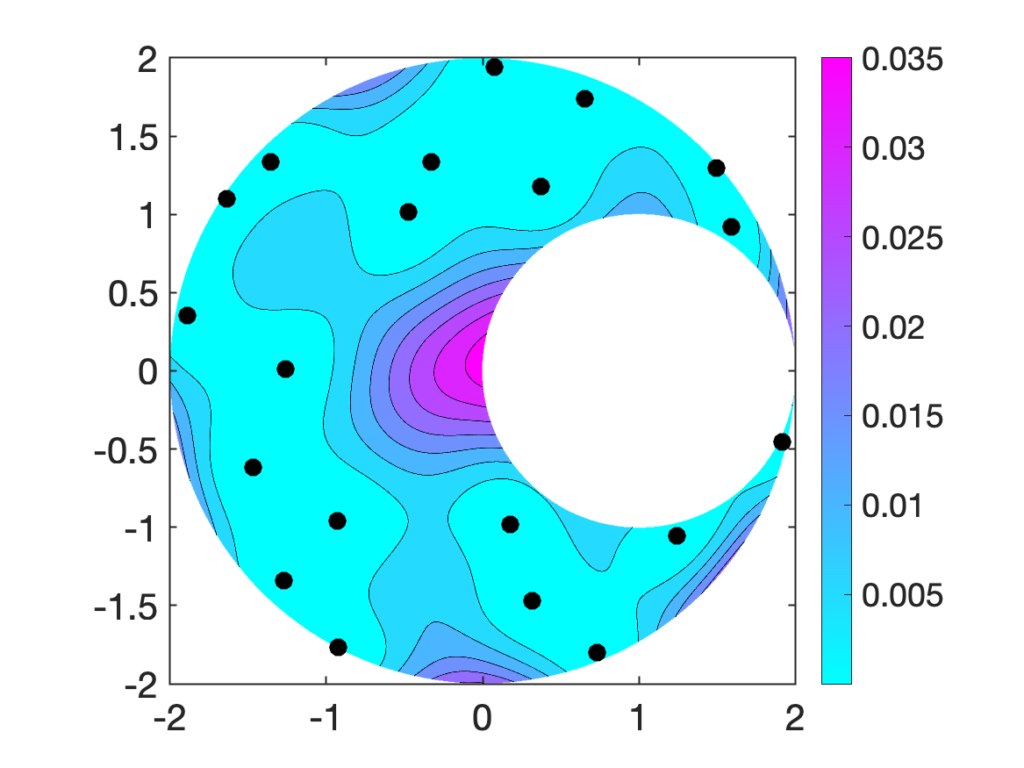
The following image shows 20 nodes selected by randomly pivoted Cholesky in a crescent-shaped region. The cyan–pink shading denotes the probability distribution for picking the next node. We see that the center of the crescent does not have any nodes, and thus is most likely to receive a node during the next round of sampling.

In our paper, we demonstrate—empirically and theoretically—that randomly pivoted Cholesky produces excellent nodes for quadrature. We also discuss efficient rejection sampling algorithms for sampling nodes with the randomly pivoted Cholesky distribution. Check out the paper for details!

Integration and Quadrature

Smoothness and Reproducing Kernel Hilbert Spaces

The Ideal Weights

Interpretation 1: Exactness

Interpretation 2: Interpolate and Integrate

Interpretation 3: Minimizing the Worst-Case Error

Interpretation 4: Minimizing the Mean-Square Error

Interpretation 5: Conditional Expectation

Conclusion

What About the Nodes?

Leave a Reply Cancel reply