Randomized Kaczmarz is Asympotically Unbiased for Least Squares

I am delighted to share that my paper Randomized Kaczmarz with tail averaging, joint with Gil Goldshlager and Rob Webber, has been posted to arXiv. This paper in particular really benefited from a lot of feedback from discussions with friends, colleagues, and experts, and I’d like to thank everyone who gave us feedback on this paper.

In this post, I want to provide a different and complementary perspective on the results of this paper, and provide some more elementary results and derivations that didn’t make the main paper.

The randomized Kaczmarz (RK) method is an iterative method for solving systems of linear equations $Ax = b$ , whose dimensions will be $n\times d$ throughout this post. Beginning from a trivial initial solution $x_0=0$ , the method works by repeating the following two steps for $t = 0,1,2,\ldots$ :

Randomly sample a row $i_t$ of $A$ with probability
$\prob\{ i_t = j\} = \frac{\norm{a_j}^2}{\norm{A}_{\rm F}^2}.$
Throughout this post, $a_j^\top$ denotes the $j$ th row of $A$ .
Orthogonally project $x_t$ onto the solution space of the equation $a_{i_t}^\top x = b_{i_t}$ , obtaining $x_{t+1} \coloneqq x_t + (b_{i_t} - a_{i_t}^\top x_t)/\norm{a_{i_t}}^2\cdot a_{i_t}$ .

The main selling point of RK is that it only interacts with the matrix $A$ through row accesses, which makes the method ideal for very large problems where only a few rows of $A$ can fit in memory at a time.

When applied to a consistent system of linear equations (i.e., a system possessing a solution $x_\star$ satisfying $Ax_\star = b$ ), RK is geometrically convergent:

(1) $\expect\left[ \norm{x_t - x_\star}^2 \right] \le (1 - \kappa_{\rm dem}^{-2})^t \norm{x_\star}^2.$

Here,

(2) $\kappa_{\rm dem} = \frac{\norm{A}_{\rm F}}{\sigma_{\rm min}(A)} = \sqrt{\sum_i \left(\frac{\sigma_i(A)}{\sigma_{\rm min}(A)}\right)^2}$

is known as the Demmel condition number, and $\sigma_i(A)$ are the singular values of $A$ .¹ However, for inconsistent problems, RK does not converge at all. Indeed, since each step of RK updates the iterate $x_t$ such that an equation $a_{i_t}^\top x = b_{i_t}$ hold exactly and no solution $x_\star$ satisfies all the equations simultaneously, the RK iterates continue to stochastically fluctuate no matter how long the algorithm is run.

However, while the RK iterates continue to randomly fluctuate when applied to an inconsistent system, their expected value does converge. In fact, it converges to the least-squares solution² $x_\star$ to the system, defined as

$x_\star = \operatorname{argmin}_{x \in \real^d} \norm{b - Ax}.$

Put differently, the bias of the RK iterates $x_t$ as estimators to the least-squares solution $x_\star$ converge to zero, and the rate of convergence is geometric. Specifically, we have the following theorem:

Theorem 1 (Exponentially Decreasing Bias): The RK iterates $x_t$ have an exponentially decreasing bias
(3) $\norm{\mathbb{E}[x_t] - x_\star}^2 \le (1 - \kappa_{\rm dem}^{-2})^{2t} \norm{x_\star}^2.$

Observe that the rate of convergence (3) for the bias is twice as fast as the rate of convergence for the error in (1). This factor of two was previously observed by Gower and Richtarik in the context of consistent systems of equations.

The proof of Theorem 1 is straightforward, and we will present it at the bottom of this post. First, we will discuss a couple of implications. First, we develop convergent versions of the RK algorithm using tail averaging. Second, we explore what happens when we implement RK with different sampling probabilities $\prob \{i_t = j\}$ .

Tail Averaging

It may seem like Theorem 1 has little implication for practice. After all, just because the expected value of $x_t$ becomes closer and closer to $x_\star$ , it need not be the case that $x_t$ is close to $x$ . However, we can improve the quality of the approximate solution $x_t$ by averaging.

There are multiple different possible ways we could use averaging. A first idea would be to run RK multiple times, obtaining multiple solutions $x^{(1)}_t,\ldots,x^{(m)}_t$ which could then be averaged together. This approach is inefficient as each solution $x_t^{(i)}$ is computed separately.

A better strategy is tail averaging. Fix a burn-in time $t_{\rm b}$ , chosen so that the bias $\norm{\expect[x_{t_{\rm b}}] - x_\star}$ is small. For each $s> t_{\rm b}$ , $x_s$ is a nearly unbiased approximation to the least-squares solution $x_\star$ . To reduce variance, we can average these estimators together

$\overline{x}_t = \frac{x_{t_{\rm b} +1} + x_{t_{\rm b}+2} + \cdots + x_t}{t-t_{\rm b}}.$

The estimator $\overline{x}_t$ is the tail-averaged randomized Kaczmarz (TARK) estimator. By Theorem 1, we know the TARK estimator has an exponentially small bias:

$\norm{\expect[\overline{x}_t] - x_\star} \le (1 - \kappa_{\rm dem}^{-2})^{2(t_{\rm b}+1)} \norm{x_\star}^2.$

In our paper, we also prove a bound for the mean-square error:

$\expect [\norm{\overline{x}_t - x_\star}^2] \le (1-\kappa_{\rm dem}^{-2})^{t_{\rm b}+1} \norm{x_\star}^2 + \frac{2\kappa_{\rm dem}^4}{t-t_{\rm b}} \frac{\norm{b-Ax_\star}^2}{\norm{A}_{\rm F}^2}.$

We see that the rate of convergence is geometric in the burn-in time $t_{\rm b}$ and occurs at an algebraic, Monte Carlo, rate in the final time $t$ . While the Monte Carlo rate of convergence may be unappealing, it is known that this rate of convergence is optimal for any method that accesses row–entry pairs $(a_i,b_i)$ ; see our paper for a new derivation of this fact.

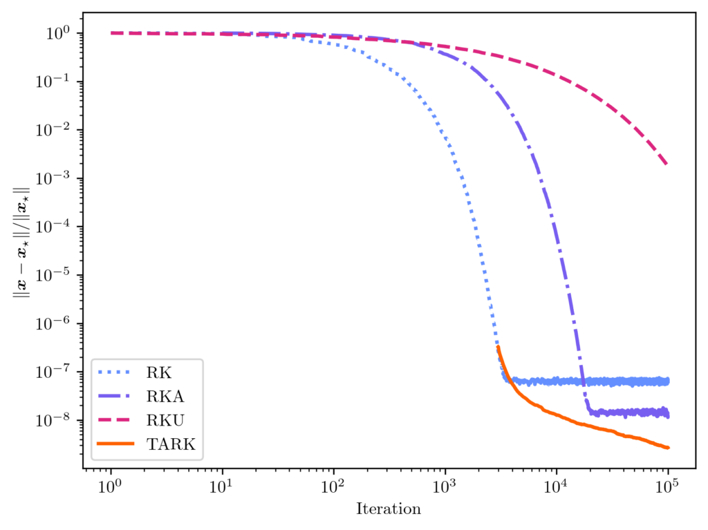
Tail averaging can be an effective method for squeezing a bit more accuracy out of the RK method for least-squares problems. The figure below shows the error of different RK methods applied to a random least-squares problem, including plain RK, RK with thread averaging (RKA), and RK with underrelaxation (RKU);³ see the paper’s Github for code. For this problem, tail-averaged randomized Kaczmarz achieves the lowest error of all of the methods considered, being 6× smaller than RKA, 22× smaller than RK, and 10⁶× smaller than RKU.

Error versus iteration for different randomized Kaczmarz methods. Tail-averaged randomized Kaczmarz shows the lowest error

What Least-Squares Solution Are We Converging To?

A second implication of Theorem 1 comes from reanalyzing the RK algorithm if we change the sampling probabilities. Recall that the standard RK algorithm draws random row indices $i_t$ using squared row norm sampling:

$\prob \{ i_t = j \} = \frac{\norm{a_j}^2}{\norm{A}_{\rm F}^2} \eqqcolon p^{\rm RK}_j.$

We have notated the RK sampling probability for row $j$ as $p_j^{\rm RK}$ .

Using the standard RK sampling procedure can sometimes be difficult. To implement it directly, we must make a full pass through the matrix to compute the sampling probabilities.⁴ It can be much more convenient to sample rows $i_t$ uniformly at random $\prob \{ i_t = j \} = 1/n$ .

To do the following analysis in generality, consider performing RK using general sampling probabilities $p_j$ :

$\prob \{i_t = j\} = p_j.$

What happens to the bias of the RK iterates then?

Define a diagonal matrix

$D \coloneqq \diag\left( \sqrt{\frac{p_j}{p_j^{\rm RK}}} : j =1,\ldots,n\right).$

One can check that the RK algorithm with non-standard sampling probabilities $\{p_j\}$ is equivalent to the standard RK algorithm run on the diagonally reweighted least-squares problem

$x_{\rm weighted} = \argmin_{x\in\real^d} \norm{Db-(DA)x}.$

In particular, applying TARK with uniform sampling probabilities, the tail-averaged iterates $\overline{x}_t$ will converge to the weighted least-squares problem $x_{\rm weighted}$ rather than the original least-squares solution $x_\star$ .

I find this very interesting. In the standard RK method, the squared row norm sampling distribution is chosen to ensure rapid convergence of the RK iterates to the solution of a consistent system of linear equations. However, for a consistent system, the RK method will always converge to the same solution no matter what row sampling strategy is chosen (as long as every non-zero row has a positive probability of being picked). In the least-squares context, however, the conclusion is very different: the choice of row sampling distribution not only affects the rate of convergence, but also which solution is being converged to!

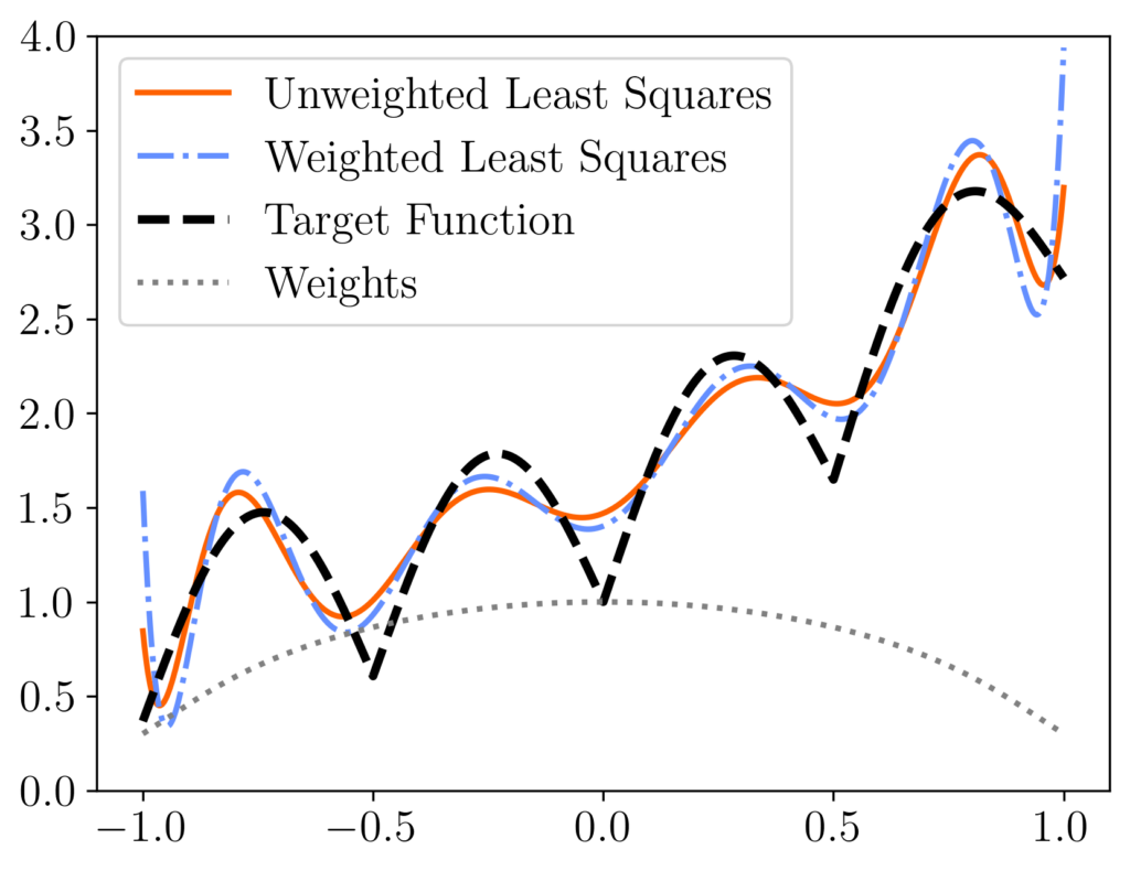
As the plot below demonstrates, the original least-squares solution and re-weighted least-squares solution can sometimes be quite different from each other. This plot shows the results of fitting a function with many kinks (show as a black dashed curve) using a polynomial function $p(u) = \sum_{j=0}^{10} x_j u^j$ [mfn}Note that, for this experiment we represent the polynomial $p(u) = \sum_{i=0}^{10} x_j u^j$ using its monomial coefficients $x_j$ , which has issues with numerical stability. It’s better to use a representation using Chebyshev polynomials. We use this example only to illustrate the difference between the weighted and original least-squares solution.[/mfn} at $10000$ equispaced points. We compare the unweighted least-squares solution (orange solid curve) to the weighted least-squares solution using uniform RK weights $p_j = 1/n$ (blue dash-dotted curve). These two curves differ meaningfully, with the weighted least-squares solution having higher error at the ends of the interval but more accuracy in the middle. These differences can be explained looking at the weights (diagonal entries of $D$ , grey dotted curve), which are lower at the ends of the interval than in the center.

Weighted and un-weighted least-squares solution to polynomial regression problem. (Tail averaged) randomized Kaczmarz method with uniform sampling converges to the weighted least-squares solution, which is more accurate on the middle of the interval (where the weights are high) than the edges of the interval (where the weights are smaller)

Does this diagonal rescaling issue matter? Sometimes not. In many applications, the weighted and un-weighted least squares solutions will both be fine. Indeed, in the above example, neither the weighted nor un-weighted solutions are the “right” one; the weighted solution is more accurate in the interior of the domain and less accurate at the boundary. However, sometimes getting the true least-squares solution matters, or the amount of reweighting done by uniform sampling is too aggressive for a problem. In these cases, using the classical RK sampling probabilities may be necessary. Fortunately, rejection sampling can often be used to perform squared row norm sampling; see this blog post of mine for details.

Proof of Theorem 1

Let us now prove Theorem 1, the asymptotic unbiasedness of randomized Kaczmarz. We will assume throughout that $A$ is full-rank; the rank-deficient case is similar but requires a bit more care.

Begin by rewriting the update rule in the following way

$x_{t+1} = \left( I - \frac{a_{i_t}^{\vphantom{\top}}a_{i_t}^\top}{\norm{a_{i_t}}^2} \right)x_t + \frac{b_{i_t}a_{i_t}}{\norm{a_{i_t}}^2}.$

Now, letting $\expect_{i_t}$ denote the average over the random index $i_t$ , we compute

$\begin{align*}\expect_{i_t}[x_{t+1}] &= \sum_{j=1}^n \left[\left( I - \frac{a_j^{\vphantom{\top}} a_j^\top}{\norm{a_j}^2} \right)x_t + \frac{b_ja_j}{\norm{a_j}^2}\right] \prob\{i_t=j\}\\ &=\sum_{j=1}^n \left[\left( \frac{\norm{a_j}^2}{\norm{A}_{\rm F}^2}I - \frac{a_j^{\vphantom{\top}} a_j^\top}{\norm{A}_{\rm F}^2} \right)x_t + \frac{b_ja_j}{\norm{A}_{\rm F}^2}\right].\end{align*}$

We can evaluate the sums $\sum_{j=1}^n a_j^{\vphantom{\top}}a_j^\top = A^\top A$ and $\sum_{j=1}^n b_j a_j = A^\top b$ directly. Therefore, we obtain

$\expect_{i_t}[x_{t+1}] = \left( I - \frac{A^\top A}{\norm{A}_{\rm F}^2}\right) x_t + \frac{A^\top b}{\norm{A}_{\rm F}^2}.$

Thus, taking the (total) expectation of both sides, we get

$\expect[x_{t+1}] = \left( I - \frac{A^\top A}{\norm{A}_{\rm F}^2}\right) \expect[x_t] + \frac{A^\top b}{\norm{A}_{\rm F}^2}.$

Iterating this equation and using the initial condition $x_0 = 0$ , we obtain

(4) $\expect[x_t] = \left[\sum_{i=0}^{t-1} \left( I - \frac{A^\top A}{\norm{A}_{\rm F}^2}\right)^i \right]\cdot\frac{A^\top b}{\norm{A}_{\rm F}^2}.$

The equation (4) expresses the expected RK iterate $\expect[x_t]$ using a matrix geometric series. Recall that the infinite geometric series with a scalar ratio $|y|<1$ satisfies the formula

$\sum_{i=0}^\infty y^i = (1-y)^{-1}.$

Substituting $x=1-y$ , we get

$\sum_{i=0}^\infty (1-x)^i = x^{-1}$

for any $0 < x < 2$ . With a little effort, one can check that the same formula

$\sum_{i=0}^\infty (I-X)^i = X^{-1}$

for a square matrix $X$ satisfying $0 < \sigma_{\rm min}(X) \le \norm{X} < 2$ . These conditions hold for the matrix $X = A^\top A / \norm{A}_{\rm F}^2$ since $A$ is full-rank, yielding

(5) $\left(\frac{A^\top A}{\norm{A}_{\rm F}^2}\right)^{-1} = \sum_{i=0}^\infty \left( I - \frac{A^\top A}{\norm{A}_{\rm F}^2}\right)^i.$

In anticipation of plugging this result into (4), we can break the infinite sum on the right-hand side into two pieces:

(6) $\left(\frac{A^\top A}{\norm{A}_{\rm F}^2}\right)^{-1} = \sum_{i=0}^{t-1} \left( I - \frac{A^\top A}{\norm{A}_{\rm F}^2}\right)^i + \sum_{i=t}^\infty \left( I - \frac{A^\top A}{\norm{A}_{\rm F}^2}\right)^i.$

We are at the home stretch. Plugging (6) into (4) and using the normal equations $x_\star = (A^\top A)^{-1} A^\top b$ , we obtain

$\expect[x_t] = x_\star - \left[\sum_{i=t}^\infty \left( I - \frac{A^\top A}{\norm{A}_{\rm F}^2}\right)^i \right]\cdot\frac{A^\top b}{\norm{A}_{\rm F}^2}.$

Rearrange to obtain

$\expect[x_t] - x_\star = - \left(I - \frac{A^\top A}{\norm{A}_{\rm F}^2}\right)^t \left[\sum_{i=0}^\infty \left( I - \frac{A^\top A}{\norm{A}_{\rm F}^2}\right)^i \right]\cdot\frac{A^\top b}{\norm{A}_{\rm F}^2}.$

Now apply (5) and the normal equations again to obtain

$\expect[x_t] - x_\star = - \left(I - \frac{A^\top A}{\norm{A}_{\rm F}^2}\right)^t x_\star.$

Take norms and use the submultiplicative property of the spectral norm to obtain

(7) $\norm{\expect[x_t] - x_\star}^2 \le \norm{I - \frac{A^\top A}{\norm{A}_{\rm F}^2}}^{2t} \norm{x}_\star^2.$

To complete the proof we must evaluate the norm of the matrix $I - A^\top A / \norm{A}_{\rm F}^2$ . Let $A = U \Sigma V^\top$ be a (thin) singular value decomposition, where $\Sigma = \diag(\sigma_{\rm max}(A),\ldots,\sigma_{\rm min}(A))$ . Then

$I - \frac{A^\top A}{\norm{A}_{\rm F}^2} = I - V \cdot\frac{\Sigma^2}{\norm{A}_{\rm F}^2} \cdot V^\top = V \left( I - \frac{\Sigma^2}{\norm{A}_{\rm F}^2}\right)V^\top.$

We recognize this as a matrix whose eigenvectors are $V$ and whose eigenvalues are the diagonal entries of the matrix

$I - \Sigma^2/\norm{A}_{\rm F}^2 = \diag(1 - \sigma^2_{\rm max}(A)/\norm{A}_{\rm F}^2,\ldots,1-\sigma_{\rm min}^2(A)/\norm{A}_{\rm F}^2).$

All eigenvalues are nonnegative and the largest eigenvalue is $1 - \sigma_{\rm min}^2(A)/\norm{A}_{\rm F}^2 = 1 - \kappa_{\rm dem}^{-2}$ . We have invoked the definition of the Demmel condition number (2). Therefore, plugging into (7), we obtain

$\norm{\expect[x_t] - x_\star}^2 \le \left(1-\kappa_{\rm dem}^{-2}\right)^{2t} \norm{x}_\star^2,$

as promised.

Tail Averaging

What Least-Squares Solution Are We Converging To?

Proof of Theorem 1

Leave a Reply Cancel reply