Vandermonde Matrices are Merely Exponentially Ill-Conditioned

August 13, 2025 by Ethan N. Epperly Leave a comment

I am excited to share that my paper Does block size matter in randomized block Krylov low-rank approximation? has recently been released on arXiv. In that paper, we study the randomized block Krylov iteration (RBKI) algorithm for low-rank approximation. Existing results show that RBKI is efficient at producing rank- $k$ approximations with a large block size of $k$ or a small block size of $1$ , but these results give poor results for intermediate block sizes $1\ll b \ll k$ . But often these intermediate block sizes are the most efficient in practice. In our paper, we close this theoretical gap, showing RBKI is efficient for any block size $1\le b \le k$ . Check out the paper for details!

In our paper, the core technical challenge is understanding the condition number of a random block Krylov matrix of the form

$K = \begin{bmatrix} G & AG & \cdots & A^{t-1}G \end{bmatrix},$

where $A$ is an $n\times n$ real symmetric positive semidefinite matrix and $G$ is an $n\times (n/b)$ random Gaussian matrix. Proving this result was not easy, and our proof required several ingredients. In this post, I want to talk about just one of them: Gautschi’s bound on the conditioning of Vandermonde matrices. (Check out Gautschi’s original paper here.)

Evaluating a Polynomial and Vandermonde Matrices

Let us begin with one the humblest but most important characters in mathematics, the univariate polynomial

$p_a(u) = a_1 + a_2 u+ \cdots + a_t u^{t-1}.$

Here, we have set the degree to be $t-1$ and have written the polynomial $p_a(\cdot)$ parametrically in terms of its vector of coefficients $a = (a_1,\ldots,a_t)$ . The polynomials of degree at most $t-1$ form a linear space of dimension $t$ , and the monomials $1,u,\ldots,u^{t-1}$ provide a basis for this space. In this post, we will permit the coefficients $a \in \complex^t$ to be complex numbers.

Given a polynomial, we often wish to evaluate it at a set of inputs. Specifically, let $\lambda_1,\ldots,\lambda_s \in \complex$ be $s$ (distinct) input locations. If we evaluate $p_a$ at each number, we obtain a list of (output) values, which we denote by $f = (p_a(\lambda_1),\ldots,p_a(\lambda_s))$ of $s$ (distinct) values, each of which given by the formula

$p_a(\lambda_i) = \sum_{j=1}^t \lambda_i^{j-1} a_j.$

Observe that the outputs $f$ are a nonlinear function of the input values $\lambda$ but a linear function of the coefficients $a$ . We may call the mapping $a \mapsto f$ the coefficients-to-values map.

Every linear transformation between vectors can be realized as a matrix–vector product, and the matrix for the coefficients-to-values map is called a Vandermonde matrix $V$ . It is given by the formula

$V= \begin{bmatrix} 1 & \lambda_1 & \lambda_1^2 & \cdots & \lambda_1^{t-1} \\ 1 & \lambda_2 & \lambda_2^2 & \cdots & \lambda_2^{t-1} \\ 1 & \lambda_3 & \lambda_3^2 & \cdots & \lambda_3^{t-1} \\ \vdots & \vdots & \vdots & \ddots & \vdots \\ 1 & \lambda_s & \lambda_s^2 & \cdots & \lambda_s^{t-1} \end{bmatrix} \in \complex^{s\times t}.$

The Vandermonde matrix defines the coefficients-to-values map in the sense that $f = Va$ .

Interpolating by a Polynomial and Inverting a Vandermonde Matrix

Going forward, let us set $s = t$ so the number of locations $\lambda = (\lambda_1,\ldots,\lambda_t)$ equals the number of coefficients $a = (a_1,\ldots,a_t)$ . The Vandermonde matrix maps the vector of coefficients $a$ to the vector of values $f = (f_1,\ldots,f_t) = (p_a(\lambda_1),\ldots,p_a(\lambda_t))$ . Its inverse $V^{-1}$ maps a set of values $f$ to a set of coefficients $a$ defining a polynomial $p_a$ which interpolates the values $f$ :

$p_a(\lambda_i) = f_i \quad \text{for } i =1,\ldots,t .$

More concisely, multiplying the inverse of a Vandermonde matrix solves the problem of polynomial interpolation.

To solve the polynomial interpolation problem with Vandermonde matrices, we can do the following. Given values $f$ , we first solve the linear system of equations $Va = f$ , obtaining a vector of coefficients $a = V^{-1}f$ . Then, define the interpolating polynomial

(1) $q(u) = a_1 + a_2 u + \cdots + a_t u^{t-1} \quad \text{with } a = V^{-1} f.$

The polynomial $q$ interpolates the values $f$ at the locations $\lambda_i$ , $q(\lambda_i) = p_a(\lambda_i) = f_i$ .

Lagrange Interpolation

Inverting a the Vandermonde matrix is one way to solve the polynomial interpolation problem, but the polynomial interpolation can also be solved directly. To do so, first notice that we can construct a special polynomial $(u - \lambda_2)(u - \lambda_3)\cdots(u-\lambda_t)$ that is zero at the locations $\lambda_2,\ldots,\lambda_t$ but nonzero at the first location $\lambda_1$ . (Remember that we have assumed that $\lambda_1,\ldots,\lambda_t$ are distinct.) Further, by rescaling this polynomial to

$\ell_1(u) = \frac{(u - \lambda_2)(u - \lambda_3)\cdots(u-\lambda_t)}{(\lambda_1 - \lambda_2)(\lambda_1 - \lambda_3)\cdots(\lambda_1-\lambda_t)},$

we obtain a polynomial whose value at $\lambda_1$ can be set to $1$ . Likewise, for each $i$ , we can define a similar polynomial

(2) $\ell_i(u) = \frac{(u - \lambda_1)\cdots(u-\lambda_{i-1}) (u-\lambda_{i+1})\cdots(u-\lambda_t)}{(\lambda_i - \lambda_1)\cdots(\lambda_i-\lambda_{i-1}) (\lambda_i-\lambda_{i+1})\cdots(\lambda_i-\lambda_t)},$

which is $1$ at $\lambda_i$ and zero at $\lambda_j$ for $j\ne i$ . Using the Dirac delta symbol, we may write

$\ell_i(\lambda_j) = \delta_{ij} = \begin{cases} 1, & i = j, \\ 0, & i\ne j. \end{cases}$

The polynomials $\ell_i$ are called the Lagrange polynomials of the locations $\lambda_1,\ldots,\lambda_q$ . Below is an interactive illustration of the second Lagrange polynomial $\ell_2$ associated with the points $\lambda_i = i$ (with $t = 5$ ).

With the Lagrange polynomials in hand, the polynomial interpolation problem is easy. To obtain a polynomial whose values are $f$ , simply multiply each Lagrange polynomial $\ell_i$ by the value $f_i$ and sum up, obtaining

$q(u) = \sum_{i=1}^t f_i \ell_i(u).$

The polynomial $q$ interpolates the values $f$ . Indeed,

(3) $q(\lambda_j) = \sum_{i=1}^t f_i \ell_i(\lambda_j) = \sum_{i=1}^t f_i \delta_{ij} = f_j.$

The interpolating polynomial computed is shown in the interactive display below:

From Lagrange to Vandermonde via Elementary Symmetric Polynomials

We now have two ways of solving the polynomial interpolation problem, the Vandermonde way (1) and the Lagrange way (3). Ultimately, the difference between these formulas is one of basis: The Vandermonde formula (1) expresses the interpolating polynomial $q$ as a linear combination of monomials $1,u,\ldots,u^{t-1}$ and the Lagrange formula (3) expresses $q$ as a linear combination of the Lagrange polynomials $\ell_1,\ldots,\ell_n$ . To convert between these formulas, we just need to express the Lagrange polynomial basis in the monomial basis.

To do so, let us examine the Lagrange polynomials more closely. Consider first the case $t = 4$ , and consider the fourth unnormalized Lagrange polynomial

$(u - \lambda_1) (u - \lambda_2) (u - \lambda_3).$

Expanding this polynomial in the monomials $u^i$ , we obtain the expression

$(u - \lambda_1) (u - \lambda_2) (u - \lambda_3) = u^3 - (\lambda_1 + \lambda_2 + \lambda_3) u^2 + (\lambda_1\lambda_2 + \lambda_1\lambda_3 + \lambda_2\lambda_3)u - \lambda_1\lambda_2\lambda_3.$

Looking at the coefficients of this polynomial in $u$ , we recognize some pretty distinctive expressions involving the $\lambda_i$ ‘s:

$\begin{align*}\text{coefficient of $u^2$} &= - (\lambda_1 + \lambda_2 + \lambda_3), \\\text{coefficient of $u$} &= \lambda_1\lambda_2 + \lambda_1\lambda_3 + \lambda_2\lambda_3, \\\text{coefficient of $1$} &= -\lambda_1\lambda_2\lambda_3.\end{align*}$

Indeed, these expressions are special. Up to a plus-or-minus sign, they are called the elementary symmetric polynomials of the locations $\lambda_i$ . Specifically, given numbers $\mu_1,\ldots,\mu_s$ , the $k$ th elementary symmetric polynomial $e_k(\mu_1,\ldots,\mu_s)$ is defined as the sum of all products $\mu_{i_1} \mu_{i_2} \cdots \mu_{i_k}$ of $k$ values, i.e.,

$e_k(\mu_1,\ldots,\mu_{t-1}) = \sum_{i_1 < i_2 < \cdots < i_k} \mu_{i_1}\mu_{i_2}\cdots \mu_{i_k}.$

The zeroth elementary symmetric polynomial is $1$ by convention.

The elementary symmetric polynomials appear all the time in mathematics. In particular, they are the coefficients of the characteristic polynomial of a matrix and feature heavily in the theory of determinantal point processes. For our purposes, the key observation will be that the elementary symmetric polynomials appear whenever one expands out an expression like $(u + \mu_1) \cdots (u + \mu_k)$ :

Lemma 1 (Expanding a product of linear functions). It holds that
$(u + \mu_1) (u + \mu_2) \cdots (u+\mu_k) = \sum_{j=0}^k e_{k-j}(\mu_1,\ldots,\mu_k) u^j.$

Using this fact, we obtain an expression for the Lagrange polynomials in the monomial basis. Let $\lambda_{-i} = (\lambda_1,\ldots, \lambda_{i-1},\lambda_{i+1},\ldots,\lambda_t)$ denote the list of locations without $\lambda_i$ . Then the $i$ th Lagrange polynomial is given by

$\ell_i(u) = \frac{\sum_{j=1}^t e_{t-j}(-\lambda_{-i})u^{j-1}}{\prod_{k\ne i} (\lambda_i - \lambda_k)}.$

Not exactly a beautiful expression, but it will get the job done.

Indeed, we can write the interpolating polynomial as

$q(u) = \sum_{i=1}^t f_i\ell_i(u) = \sum_{i=1}^t \sum_{j=1}^t f_i \frac{e_{t-j}(-\lambda_{-i})}{\prod_{k\ne i} (\lambda_i - \lambda_k)} u^{j-1}.$

To make progress, we interchange the order of summation and regroup:

$q(u) = \sum_{j=1}^t \sum_{i=1}^t f_i \frac{e_{t-j}(-\lambda_{-i})}{\prod_{k\ne i} (\lambda_i - \lambda_k)} u^{j-1} = \sum_{j=1}^t \left(\sum_{i=1}^t \frac{e_{t-j}(-\lambda_{-i})}{\prod_{k\ne i} (\lambda_i - \lambda_k)}\cdot f_i \right) u^{j-1}.$

We see that the coefficients of the interpolating polynomial (in the monomial basis) are

$a_j = \sum_{i=1}^t \frac{e_{t-j}(-\lambda_{-i})}{\prod_{k\ne i} (\lambda_i - \lambda_k)}\cdot f_i.$

But we also know that the coefficients are given by $a = V^{-1}f$ . Therefore, we conclude that the entries of the inverse-Vandermonde matrix $V^{-1}$ are

(4) $(V^{-1})_{ji} = \frac{e_{t-j}(-\lambda_{-i})}{\prod_{k\ne i} (\lambda_i - \lambda_k)}.$

Vandermonde Matrices are Merely Exponentially Ill-Conditioned

Vandermonde matrices are notoriously ill-conditioned, meaning that small changes to the values $f$ can cause large changes to the coefficients $a$ . On its face, this might seem like the problem of polynomial interpolation itself is ill-conditioned, but this is too hasty a conclusion. After all, it is only the mapping from values $f$ to coefficients $a$ in the monomial basis that is ill-conditioned. Fortunately, there are much better, more numerically stable bases for representing a polynomial like the Chebyshev polynomials.

But these more stable methods of polynomial interpolation and approximation are not the subject of this post: Here, our task is to will be to characterize just how ill-conditioned the computation of $a = V^{-1}f$ is. To characterize this ill-conditioning, we will utilize the condition number of the matrix $V$ . Given a norm $\uinorm{\cdot}$ , the condition number of $V$ is defined to be

$\kappa_{\uinorm{\cdot}}(V) = \uinorm{V} \uinorm{\smash{V^{-1}}}.$

For this post, we will focus on the case where $\uinorm\cdot}$ is chosen to be the (operator) $1$ –norm, defined as

$\norm{A}_1= \max_{x \ne 0} \frac{\norm{Ax}_1}{\norm{x}_1} \quad \text{where } \norm{x}_1 = \sum_i |x_i|.$

The $1$ -norm has a simple characterization: It is the maximum sum of the absolute values of the entries in any column

(5) $\norm{A}_\infty = \max_j \sum_i |A_{ij}|.$

We shall denote the $1$ -norm condition number $\kappa_1(\cdot)$ .

Bounding $\norm{V}_1$ is straightforward. Indeed, setting $M = \max_{1\le i \le t} |\lambda_i|$ and using (5), we compute

$\norm{V}_1= \max_{1\le j \le t} \sum_{i=1}^t |\lambda_i|^{j-1} \le \max_{1\le j \le t} tM^{j-1} = t\max\{1,M^{t-1}\}.$

An even weaker, but still useful, bound is

$\norm{V}_1\le t(1+M)^{t-1}.$

The harder task is bounding $\norm{\smash{V^{-1}}}_1$ . Fortunately, we have already done most of the hard work needed to bound this quantity. Using our expression (4) for the entries of $V^{-1}$ and using the formula (5) for the $1$ -norm, we have

$\norm{\smash{V^{-1}}}_1= \max_{1\le j \le t} \sum_{i=1}^t |(V^{-1})_{ij}| = \max_{1\le j \le t}\frac{ \sum_{i=1}^t |e_{t-i}(-\lambda_{-j})|}{\prod_{k\ne j} |\lambda_j- \lambda_k|}.$

To bound this expression, we make use of the following “triangle inequality” for elementary symmetric polynomials

$|e_k(\mu_1,\ldots,\mu_s)| \le e_k(|\mu_1|,\ldots,|\mu_s|).$

Using this bound and defining $|\lambda_{-j}| = (|\lambda_1|,\ldots,|\lambda_{j-1}|,|\lambda_{j+1}|,\ldots,|\lambda_t|)$ , we obtain

$\norm{\smash{V^{-1}}}_1\le \max_{1\le j \le t}\frac{ \sum_{i=1}^t e_{t-i}(|\lambda_{-j}|)}{\prod_{k\ne j} |\lambda_j- \lambda_k|}.$

We now use the Lemma 1 with $u = 1$ to obtain the expression

(6) $\norm{\smash{V^{-1}}}_1\le \max_{1\le j \le t}\frac{ \prod_{k\ne j} (1 + |\lambda_k|)}{\prod_{k\ne j} |\lambda_j- \lambda_k|}.$

Equation (6) is Gautschi’s bound on the norm of the inverse of a Vandermonde matrix, the result we were working towards proving.

Often, it is helpful to simply Gautschi’s bound a bit. Setting $M = \max_{1\le i \le t} |\lambda_i|$ as above, the numerator is bounded as $(1+M)^{t-1}$ . To bound the denominator, let $\mathrm{gap} \coloneqq \min_{k \le j} |\lambda_j - \lambda_k|$ be the smallest distance between two locations. Using $M$ and $\mathrm{gap}$ , we can weaken the bound (6) to obtain

$\norm{\smash{V^{-1}}}_1\le \left(\frac{1+M}{\mathrm{gap}}\right)^{t-1}.$

Combining this with our bound on $\norm{V}_\infty$ from above, we obtain a bound on the condition number

$\kappa_1(V) \le t \left( \frac{(1+M)^2}{\mathrm{gap}} \right)^{t-1}.$

We record these results:

Theorem 2 (Gautschi’s bound, simplified). Introduce $M = \max_{1\le i \le t} |\lambda_i|$ and $\mathrm{gap} \coloneqq \min_{k < j} |\lambda_j - \lambda_k|$ . Then
$\norm{\smash{V^{-1}}}_1\le \left(\frac{1+M}{\mathrm{gap}}\right)^{t-1}$
and
$\kappa_1(V) \le t \left( \frac{(1+M)^2}{\mathrm{gap}} \right)^{t-1}.$

Gautschi’s bound suggests that Vandermonde matrices can be very ill-conditioned, which is disappointing. But Gautschi’s bound also shows that Vandermonde matrices are merely exponentially ill-conditioned—that is, they are not worse than exponentially conditioned. The fact that Vandermonde matrices are only exponentially ill-conditioned plays a crucial role in our analysis of randomized block Krylov iteration.

Gautschi’s Bound as a Robust Version of the Fundamental Theorem of Algebra

The fundamental theorem of algebra states that a degree- $(t-1)$ polynomial has precisely $t-1$ roots. Consequently, at $t$ locations, it must be nonzero at least one. But how nonzero must the polynomial be at that one location? How large must it be? On this subject, the fundamental theorem of algebra is moot. However, Gautschi’s bound provides an answer.

To answer this question, we ask: What is the minimum possible size $\norm{f}_1$ of the values $f = Va = (p_a(\lambda_1),\ldots,p_a(\lambda_t))$ ? Well, if we set all the coefficients $a = (0,\ldots,0)$ to zero, then $f = 0$ as well. So to avoid this trivial case, we should enforce a normalization condition on the coefficient vector $a$ , say $\norm{a}_1 = 1$ . With this setting, we are ready to compute. Begin by observing that

$\min_{\norm{a}_1 = 1} \norm{Va}_1 = \min_{a\ne 0} \frac{\norm{Va}_1}{\norm{a}_1}.$

Now, we make the change of variables $f = V^{-1}a$ , obtaining

$\min_{\norm{a}_1 = 1} \norm{Va}_1 = \min_{a\ne 0} \frac{\norm{Va}_1}{\norm{a}_1} = \min_{f\ne 0} \frac{\norm{f}_1}{\norm{\smash{V^{-1}f}}_1}.$

Now, take the inverse of both sides to obtain

$\left(\min_{\norm{a}_1 = 1} \norm{Va}_1\right)^{-1} = \max_{f\ne 0} \frac{\norm{\smash{V^{-1}f}}_1}{\norm{f}_1} = \norm{\smash{V^{-1}}}_1.$

Ergo, we conclude

$\min_{\norm{a}_1 = 1} \norm{Va}_1 = \norm{\smash{V^{-1}}}_1^{-1}.$

Indeed, this relation holds for all operator norms:

Proposition 3 (Minimum stretch). For vector norm $\uinorm{\cdot}$ and its induced operator norm $\uinorm{\cdot}$ , it holds that for any square invertible matrix $A$ that
$\min_{\uinorm{v} = 1} \uinorm{Av} = \min_{v\ne 0} \frac{\uinorm{Av}}{\uinorm{v}} = \uinorm{\smash{A^{-1}}}^{-1}.$

Using this result, we obtain the lower bound $\norm{f}_1\ge \norm{a}_1/\norm{\smash{V^{-1}}}_1$ on the values $f$ of a polynomial with coefficients $a$ . Combining with Gautschi’s bound gives the following robust version of the fundamental theorem of algebra:

Theorem 4 (Robust fundamental theorem of algebra). Fix a polynomial $p(u) = a_1 + a_2 t + \cdots + a_t u^{t-1}$ and locations $\lambda_1,\ldots,\lambda_t$ . Define $M = \max_{1\le i \le t} |\lambda_i|$ and $\mathrm{gap} \coloneqq \min_{k \le j} |\lambda_j - \lambda_k|$ . Then
$|p(\lambda_1)| + \cdots + |p(\lambda_t)| \ge \left(\frac{\mathrm{gap}}{1+M}\right)^{t-1} (|a_1| + \cdots + |a_t|).$

Thus, at $t$ locations, a degree- $(t-1)$ polynomial must be nonzero at least one point. In fact, the sum of the values at these $t$ locations must be no worse than exponentially small in $t$ .

Gaussian Integration by Parts

August 4, 2025 by Ethan N. Epperly Leave a comment

Gaussian random variables are wonderful, and there are lots of clever tricks for doing computations with them. One particularly nice tool is the Gaussian integration by parts formula, which I learned from my PhD advisor Joel Tropp. Here it is:

Gaussian integration by parts. Let $z$ be a standard Gaussian random variable. Then $\expect[zf(z)] = \expect[f'(z)]$ .

This formula makes many basic computations effortless. For instance, to compute the second moment $\expect[z^2]$ of a standard Gaussian random variable $z$ , we apply the formula with $f(x) = x$ to obtain

$\expect[z^2] = \expect[z f(z)] = \expect[f'(z)] = \expect[1] = 1.$

Therefore, the second moment is one. Since $z$ has mean zero, this also means that the variance of a standard Gaussian random variable is one.

The fourth moment is no harder to compute. Using $f(x) = x^3$ , we compute

$\expect[z^4] = \expect[zf(z)] = \expect[f'(z)] = 3\expect[z^2] = 3.$

Easy peesy. We’ve shown the fourth moment of a standard Gaussian variable is three—no fancy integral tricks required.

Iterating this trick, we can compute all the even moments of a standard Gaussian random variable. Indeed,

$\expect[z^{2p}] = \expect[z\cdot z^{2p-1}] = (2p-1) \expect[z^{2p-2}] = (2p-1)(2p-3) \expect[z^{2p-4}] = \cdots = (2p-1)(2p-3)\cdots 1.$

We conclude that the $(2p)$ th moment of a standard Gaussian random variable is $(2p-1)!!$ , where $!!$ indicates the (in)famous double factorial $(2p-1)!! = (2p-1)\times(2p-3)\times\cdots \times 3 \times 1$ .

As a spicier application, let us now compute $\expect[|z|]$ . To do so, we choose $f(x) = \operatorname{sign}(x)$ to be the sign function:

$\operatorname{sign}(x) = \begin{cases} 1, & x > 0, \\ 0 & x = 0, \\ -1 & x < 0.\end{cases}$

This function is not differentiable in a “Calculus 1” sense because it is discontinuous at zero. However, it is differentiable in a “distributional sense” and its derivative is $f'(x) = 2\delta(x)$ , where $\delta$ denotes the famous Dirac delta “function”. We then compute

$\expect[|z|] = \expect[zf(z)] = \expect[f'(z)] = 2\expect[\delta(z)].$

To compute $\expect[\delta(z)]$ , write the integral out using the probability density function $\phi$ of the standard Gaussian distribution:

$\expect[|z|] = 2\expect[\delta(z)] = 2\int_{-\infty}^\infty \phi(x) \delta(x) \, \mathrm{d} x = 2\phi(0).$

The standard Gaussian distribution has density

$\phi(x) = \frac{1}{\sqrt{2\pi}} \exp \left( - \frac{x^2}{2} \right),$

so we conclude

$\expect[|z|] = 2 \cdot \frac{1}{\sqrt{2 \pi}} = \sqrt{\frac{2}{\pi}}}.$

An unpleasant computation involving integrating against the Gaussian density has again been made trivial by using the Gaussian integration by parts formula.

Application: Power Method from a Random Start

As an application of the Gaussian integration by parts formula, we can analyze the famous power method for eigenvalue computations with a (Gaussian) random initialization. This discussion is adapted from the tutorial of Kireeva and Tropp (2024).

Setup

Before we can get to the cool application of the Gaussian integration by parts formula, we need to setup the problem and do a bit of algebra. Let $A$ be a matrix, which we’ll assume for simplicity to be symmetric and positive semidefinite. Let $\lambda_1 > \lambda_2 \ge \lambda_3 \ge \cdots \ge \lambda_n \ge 0$ denote the eigenvalues of $A$ . We assume the largest eigenvalue $\lambda_1$ is strictly larger than the next eigenvalue $\lambda_2$ .

The power method computes the largest eigenvalue of $A$ by repeating the iteration $x \gets Ax / \norm{Ax}$ . After many iterations, $x$ approaches an eigenvector of $A$ and $x^\top A x$ approaches an eigenvalue. Letting $x^{(0)}$ denote the initial vector, the $t$ th power iterate is $x^{(t)} = A^t x^{(0)} / \norm{A^t x^{(0)}}$ and the $t$ th eigenvalue estimate is

$\mu^{(t)} = \left(x^{(t)}\right)^\top Ax^{(t)}= \frac{\left(x^{(0)}\right)^\top A^{2t+1} x^{(0)}}{\left(x^{(0)}\right)^\top A^{2t} x^{(0)}}.$

It is common to initialize the power method with a vector $x^{(0)}$ with (independent) standard Gaussian random coordinates. In this case, the components $z_1,\ldots,z_n$ of $x^{(0)}$ in an eigenvector basis of $A$ are also independent standard Gaussians, owing to the rotational invariance of the (standard multivariate) Gaussian distribution. Then the $t$ th eigenvalue estimate is

$\mu^{(t)} = \frac{\sum_{i=1}^n \lambda_i^{2t+1} z_i^2}{\sum_{i=1}^n \lambda_i^{2t} z_i^2},$

and the error of $\mu^{(t)}$ as an approximation to the dominant eigenvalue $\lambda_1$ is

$\frac{\lambda_1 - \mu^{(t)}}{\lambda_1} = \frac{\sum_{i=1}^n (\lambda_1 - \lambda_i)/\lambda_1 \cdot \lambda_i^{2t} z_i^2}{\sum_{i=1}^n \lambda_i^{2t} z_i^2}.$

Analysis

Having set everything up, we can now use the Gaussian integration by parts formula to make quick work of the analysis. To begin, observe that the quantity

$\frac{\lambda_1 - \lambda_i}{\lambda_1}$

is zero for $i = 1$ and is at most one for $i > 1$ . Therefore, the error is bounded as

$\frac{\lambda_1 - \mu^{(t)}}{\lambda_1} \le \frac{\sum_{i=2}^n \lambda_i^{2t} z_i^2}{\lambda_1^{2t} z_1^2 + \sum_{i=2}^n \lambda_i^{2t} z_i^2} = \frac{c^2}{\lambda_1^{2t} z_1^2 + c^2} \quad \text{for } c^2 = \sum_{i=2}^n \lambda_i^{2t} z_i^2.$

We have introduced a parameter $c$ to consolidate the terms in this expression not depending on $z_1$ . Since $z_1,\ldots,z_n$ are independent, $z_1$ and $c$ are independent as well.

Now, let us bound the expected value of the error. First, we take an expectation $\expect_{z_1}$ with respect to only the randomness in the first Gaussian variable $z_1$ . Here, we use Gaussian integration by parts in the reverse direction. Introduce the function

$f'(x) = \frac{c^2}{\lambda_1^{2t}x^2 + c^2}.$

This function is the derivative of

$f(x) = \frac{c}{\lambda_1^t} \arctan \left( \frac{\lambda_1^t}{c} \cdot x \right).$

Thus, by the Gaussian integration by parts formula, we have

$\expect_{z_1}\left[\frac{\lambda_1 - \mu^{(t)}}{\lambda_1}\right] \le \expect_{z_1} \left[z_1 \cdot \frac{c}{\lambda_1} \arctan \left( \frac{\lambda_1^t}{c} \cdot z_1 \right) \right] = \expect_{z_1} \left[|z_1| \cdot \frac{c}{\lambda_1^t} \left|\arctan \left( \frac{\lambda_1^t}{c} \cdot z_1 \right)\right| \right].$

In the last line, we observed that the bracketed quantity is nonnegative, so we are free to introduce absolute value signs. The arctangent function is always at most $\pi/2$ , so we can bound

$\expect_{z_1}\left[\frac{\lambda_1 - \mu^{(t)}}{\lambda_1}\right] \le = \frac{\pi}{2} \cdot \frac{c}{\lambda_1^t} \cdot \expect_{z_1} \left[|z_1|\right] \le \sqrt{\frac{\pi}{2}} \cdot \frac{c}{\lambda_1^t}.$

Here, we used our result from above that $\expect[|z|] = \sqrt{2/\pi}$ for a standard Gaussian variable $z$ .

We’re in the home stretch! We can bound $c$ as

$c = \sqrt{\sum_{i=2} \lambda_i^{2t} z_i^2} \le \lambda_2^{t} \sqrt{\sum_{i=2}^n z_i^2} = \lambda_2^t \norm{(z_2,\ldots,z_n)}.$

We see that $c$ is at most $\lambda_2^t$ times the length of a vector of $n-1$ standard Gaussian entries. As we’ve seen before on this blog, the expected length of a Gaussian vector with $n-1$ entries is at most $\sqrt{n-1}$ . Thus, $\expect[c] \le \lambda_2^t \sqrt{n-1}$ . We conclude that the expected error for power iteration is

$\expect\left[\frac{\lambda_1 - \mu^{(t)}}{\lambda_1}\right] = \expect_c\left[\expect_{z_1} \left[ \frac{\lambda_1 - \mu^{(t)}}{\lambda_1} \right]\right] \le \sqrt{\frac{\pi}{2}} \cdot \expect\left[ \frac{c}{\lambda_1^t} \right] =\sqrt{\frac{\pi}{2}} \cdot \left(\frac{\lambda_2}{\lambda_1}\right)^t \cdot \sqrt{n-1} .$

We see that the power iteration converges geometrically at a rate of at least $(\lambda_2/\lambda_1)^t$ .

The first analyses of power iteration from a random start were done by Kuczyński and Woźniakowski (1992) and require pages of detailed computations involving integrals. This simplified analysis, due to Tropp (2020), makes the analysis effortless by comparison.

Five Years of Blogging

July 8, 2025 by Ethan N. Epperly 1 Comment

Five years ago today, I embarked on a crazy experiment. It was the summer after I finished my undergraduate degree, and I was filled with lots of exciting things I learned from my mentor Shiv Chandrasekaran and my own self-study. I kept asking, “Why did no one teach me that subject in this way? If Shiv hadn’t taught me this trick, how would I have ever have learned this? How does everyone not know this cool theorem?” I was young and naïve. But I also was brimming with passion for my subject, and I had a lot I wanted to say.

Applied mathematics, and mathematics in general, is a rare subject in which its best researchers are also among its best communicators. Writers like Joel Tropp, Nick Trefethen, and Nick Higham were my heroes, and I desperately wanted to be like them. I figured that practice is the best way to learn any skill, and I decided that writing a blog was the best way to hone my skills as a mathematical communicator and to share this burning list of mathematical curiosities I had collected on my travels. I had my doubts—was this a waste of my time? would anyone actually want to read this? did I really have anything worth saying?—but I pushed them aside and published my first blog post on July 8, 2020.

To my great surprise, this experiment has been a bigger success than I ever could have imagined. An early success came just a month after starting the blog when my post on Galerkin approximation was posted to Hacker news and received 18,000 page views in a few-day span: what a rush! But perhaps a bigger surprise to me was how writing the blog has helped connect me to people in my field. I can’t count how many times the blog comes up within minutes of meeting a new researcher, and—to my great shock—the blog has now started to garner citations in academic papers. To everyone who’s read this blog and gotten something out of it, thank you.

It is hard to truly internalize how much things have changed for me over the past five years of blogging. I went from incoming PhD student to PhD student to person with a PhD. I met my heroes—not just Joel Tropp, Nick Trefethen, and Nick Higham—but also many more like John Urschel, Heather Wilber, Anne Greenbaum, Yuji Nakatsuksa, and Lin Lin, to name just a few. I am honored that many of them are now my collaborators. Truly, computational mathematics is a wonderful research community, and I am proud to be a member of such a warm and inviting group. I am excited to continue my research—and blogging—later this summer as a Miller postdoctoral fellow at UC Berkeley.

Let me end with a message to my former self or anyone else thinking about writing a blog, producing a YouTube video, or creating any other type of expository content: Just start! The world is hungry for clear explanations of difficult subjects, and your unique perspective on your subject is worth sharing. Your writing might not be very good at first (mine certainly wasn’t), but you’ll improve with practice. Just start. You may be surprised where you end up.

Randomized Kaczmarz: How Should You Sample?

June 16, 2025 by Ethan N. Epperly Leave a comment

The randomized Kaczmarz method is a method for solving systems of linear equations:

(1) $\text{Find $x$ such that } Ax = b.$

Throughout this post, the matrix $A$ will have dimensions $n\times d$ . Beginning from an initial iterate $x_0 = 0$ , randomized Kaczmarz works as follows. For $t = 0,1,2,\ldots$ :

Sample a random row index $i_t$ with probability $\prob \{ i_t = j \} = p_j$ .
Update to enforce the equation $a_{i_t}^\top x = b_{i_t}$ holds exactly:
$x_{t+1} \coloneqq x_t + \frac{b_{i_t} - a_{i_t}^\top x_t}{\norm{a_{i_t}}^2} a_{i_t}.$
Throughout this post, $a_j^\top$ denotes the $j$ th row of $A$ .

What selection probabilities $p_j$ should we use? The answer to this question may depend on whether the system (1) is consistent, i.e., whether it possesses a solution $x$ . For this post, we assume (1) is consistent; see this previous post for a discussion of the inconsistent case.

The classical selection probabilities for randomized Kaczmarz were proposed by Strohmer and Vershynin in their seminal paper:

(1) $p_j = \frac{\norm{a_j}^2}{\norm{A}_{\rm F}^2} \quad \text{for } j = 1,2,\ldots,n.$

Computing these selection probabilities requires a full pass over the matrix, which can be expensive for the largest problems.¹ A computationally appealing alternative is to implement randomized Kaczmarz with uniform selection probabilities

(2) $p_j = \frac{1}{n} \quad \text{for } j = 1,2,\ldots,n.$

Ignoring computational cost, which sampling rule leads to faster convergence: (1) or (2)?

Surprisingly, to me at least, the simpler strategy (2) often works better than (1). Here is a simple example. Define a matrix $A \in \real^{20\times 20}$ with entries $A_{ij} = \min(i,j)^2$ , and choose the right-hand side $b\in\real^{20}$ with standard Gaussian random entries. The convergence of standard RK with sampling rule (1) and uniform RK with sampling rule (2) is shown in the plot below. After a million iterations, the difference in final accuracy is dramatic: the final relative error 0.00012 was uniform RK and 0.67 for standard RK!

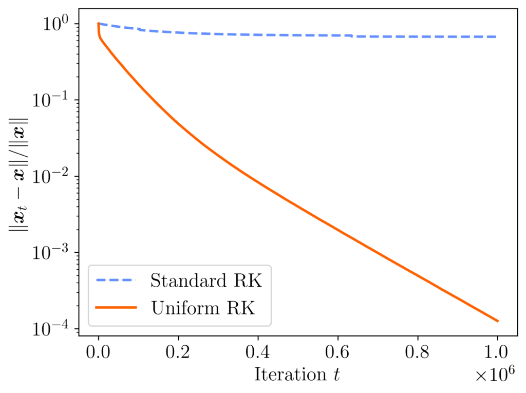
Error for randomized Kaczmarz with both squared row norm sampling ("standard") and uniformly random rows on matrix with entries min(i,j)^2. Uniform randomized Kaczmarz achieves significantly smaller final error

In fairness, uniform RK does not always outperform standard RK. If we change the matrix entries to $A_{ij} = \min(i,j)$ , then the performance of both methods is similar, with both methods ending with a relative error of about 0.07.

Error for randomized Kaczmarz with both squared row norm sampling ("standard") and uniformly random rows on matrix with entries min(i,j). Uniform randomized Kaczmarz and standard randomized Kaczmarz achieve comparable final errors

Another experiment, presented in section 4.1 of Strohmer and Vershynin’s original paper, provides an example where standard RK converges a bit more than twice as fast as uniform RK (called “simple RK” in their paper). Still, taken all together, these experiments demonstrate that standard RK (sampling probabilities (1)) is often not dramatically better than uniform RK (sampling probabilities (2)), and uniform RK can be much better than standard RK.

Randomized Kaczmarz Error Bounds

Why does uniform RK often outperform standard RK? To answer these questions, let’s look at the error bounds for the RK method.

The classical analysis of standard RK shows the method is geometrically convergent

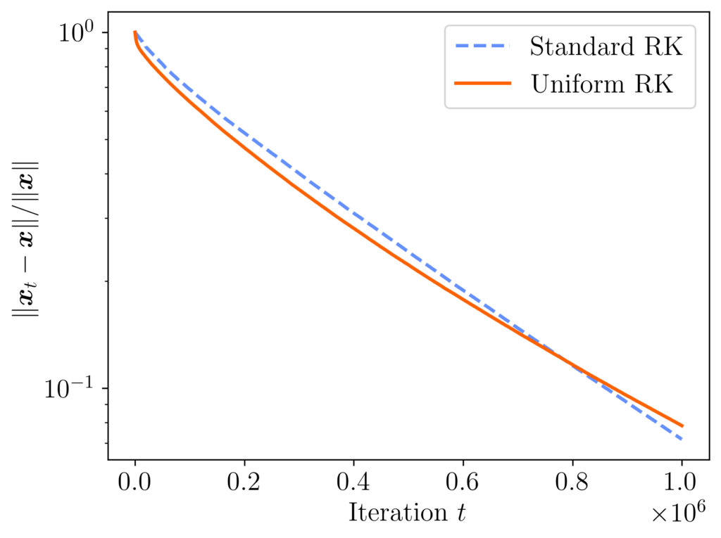
(3) $\expect\left[ \norm{x_t - x_\star}^2 \right] \le (1 - \kappa_{\rm dem}(A)^{-2})^t \norm{x_\star}^2.$

Here,

(4) $\kappa_{\rm dem}(A) = \frac{\norm{A}_{\rm F}}{\sigma_{\rm min}(A)} = \sqrt{\sum_i \left(\frac{\sigma_i(A)}{\sigma_{\rm min}(A)}\right)^2}$

is known as the Demmel condition number and $\sigma_i(A)$ are the singular values of $A$ . Recall that we have assumed the system $Ax = b$ is consistent, possessing a solution $x_\star$ . If there are multiple solutions, we let $x_\star$ denote the solution of minimum norm.

What about uniform RK? Let $D_A = \diag ( \norm{a_i}^{-1} : i=1,\ldots,n )$ denote a diagonal matrix containing the inverse row norms, and introduce the row-equilibrated matrix $D_A A$ . The row-equilibrated matrix $D_A A$ has been obtained from $A$ by rescaling each of its rows to have unit norm.

Uniform RK can then be related to standard RK run on the row-equilibrated matrix:

Fact (uniform sampling and row equilibration): Uniform RK on the system $Ax = b$ produces the same sequence of (random) iterates $\hat{x}_t$ as standard RK applied to the row-equilibrated system $(D_A A)x = D_A b$ .

Therefore, by (3), the iterates $\hat{x}_t$ of uniform RK satisfy the bound

(5) $\expect\left[ \norm{\hat{x}_t - x_\star}^2 \right] \le (1 - \kappa_{\rm dem}(D_A A)^{-2})^t \norm{x_\star}^2.$

Thus, at least using the error bounds (3) and (5), whether standard or uniform RK is better depends on which matrix has a smaller Demmel condition number: $A$ or $D_A A$ .

Row Equilibration and the Condition Number

Does row equilibration increase or decrease its condition number? What is the optimal way of scaling the rows of a matrix to minimize its condition number? These are classical questions in numerical linear algebra, and they were addressed in a classical 1969 paper of van der Sluis. These results were then summarized and generalized in Higham’s delightful monograph Accuracy and Stability of Numerical Algorithms. Here, we present answers to these questions using a variant of van der Sluis’ argument.

First, let’s introduce some more concepts and notation. Define the spectral norm condition number

$\kappa(A) \coloneqq \frac{\sigma_{\rm max}(A)}{\sigma_{\rm min}(A)}$

The spectral norm and Demmel condition numbers are always comparable $\kappa(A) \le \kappa_{\rm dem}(A)\le \sqrt{\min(n,d)}\cdot \kappa(A)$ . Also, let $\mathrm{Diag}$ denote the set of all (nonsingular) diagonal matrices.

Our first result shows us that row equilibration never hurts the Demmel condition number by much. In fact, the row-equilibrated matrix produces a nearly optimal Demmel condition number when compared to any row scaling:

Theorem 1 (Row equilibration is a nearly optimal row scaling). Let $A\in\real^{n\times d}$ be wide $n\le d$ and full-rank, and let $D_AA$ denote the row-scaling of $A$ to have unit row norms. Then
$\kappa_{\rm dem}(D_AA) \le \sqrt{n}\cdot \min_{D \in \mathrm{Diag}} \kappa (DA) \le \sqrt{n}\cdot \min_{D \in \mathrm{Diag}} \kappa_{\rm dem} (DA).$

By scaling the rows of a square or wide matrix to have unit norm, we bring the Demmel condition number to within a $\sqrt{n}$ factor of the optimal row scaling. In fact, we even bring the Demmel condition number to within a $\sqrt{n}$ factor of the optimal spectral norm condition number for any row scaling.

Since the convergence rate for randomized Kaczmarz is $\kappa_{\rm dem}(A)^{-2}$ , this result shows that implementing randomized Kaczmarz with uniform sampling yields to a convergence rate that is within a factor of $n$ of the optimal convergence rate using any possible sampling distribution.

This result shows us that row equilibration can’t hurt the Demmel condition number by much. But can it help? The following proposition shows that it can help a lot for some problems.

Proposition 2 (Row equilibration can help a lot). Let $A\in\real^{n\times d}$ be wide $n\le d$ and full-rank, and let $\gamma$ denote the maximum ratio between two row norms:
$\gamma \coloneqq \frac{ \max_i \norm{a_i}}{\min_i \norm{a_i}}.$
Then the Demmel condition number of the original matrix $A$ satisfies
$\kappa_{\rm dem}(A) \le \gamma \cdot \kappa_{\rm dem}(D_A A).$
Moreover, for every $\gamma\ge 1$ , there exists a matrix $A_\gamma$ where this bound is nearly attained:
$\kappa_{\rm dem}(A_\gamma) \ge \sqrt{1-\frac{1}{n}} \cdot \gamma \cdot \kappa_{\rm dem}(D_{A_\gamma}A_\gamma).$

Taken together, Theorem 1 and Proposition 2 show that row equilibration often improves the Demmel condition number, and never increases it by that much. Consequently, uniform RK often converges faster than standard RK for square (or short wide) linear systems, and it never converges much slower.

Proof of Theorem 1

We follow Higham’s approach. Each of the $n$ rows of $D_AA$ each have unit norm, so

(7) $\norm{D_AA}_{\rm F} = \sqrt{n}.$

The minimum singular value of $D_A A$ can be written in terms of the Moore–Penrose pseudoinverse $(D_A A)^\dagger = A^\dagger D_A^{-1}$ as follows

$\frac{1}{\sigma_{\rm min}(D_A A)} = \norm{A^\dagger D_A^{-1}}.$

Here, $\norm{\cdot}$ denotes the spectral norm. Then for any nonsingular diagonal matrix $D$ , we have

(8) $\frac{1}{\sigma_{\rm min}(D_A A)} = \norm{A^\dagger D^{-1} (DD_A^{-1})} \le \norm{A^\dagger D^{-1}} \norm{DD_A^{-1}} = \frac{\norm{DD_A^{-1}}}{\sigma_{\rm min}(DA)}.$

Since the matrix $DD_A^{-1}$ is diagonal its spectral norm is

$\norm{DD_A^{-1}} = \max \left\{ \frac{|D_{ii}|}{|(D_A)_{ii}|} : 1\le i \le n \right\}.$

The diagonal entries of $D_A$ are $\norm{a_i}^{-1}$ , so

$\norm{DD_A^{-1}} = \max \left\{ |D_{ii}|\norm{a_i} : 1\le i\le n \right\}$

is the maximum row norm of the scaled matrix $DA$ . The maximum row norm is always less than the largest singular value of $DA$ , so $\norm{DD_A^{-1}} \le \sigma_{\rm max}(DA)$ . Therefore, combining this result, (7), and (9), we obtain

$\kappa_{\rm dem}(D_AA) \le \sqrt{n} \cdot \frac{\sigma_{\rm max}(DA)}{\sigma_{\rm min}(DA)} = \sqrt{n}\cdot \kappa (DA).$

Since this bound holds for every $D \in \mathrm{Diag}$ , we are free to minimize over $D$ , leading to the first inequality in the theorem:

$\kappa_{\rm dem}(D_AA) \le \sqrt{n}\cdot \min_{D \in \mathrm{Diag}} \kappa (DA).$

Since the spectral norm condition number is smaller than the Demmel condition number, we obtain the second bound in the theorem.

Proof of Proposition 2

Write $A = D_A^{-1}(D_AA)$ . Using the Moore–Penrose pseudoinverse again, write

(10) $\kappa_{\rm dem}(A) = \norm{D_A^{-1}(D_AA)}_{\rm F} \norm{(D_A A)^\dagger D_A}.$

The Frobenius norm and spectral norm satisfy a (mixed) submultiplicative property

$\norm{BC}_{\rm F} \le \norm{B}\norm{C}_{\rm F}, \quad \norm{BC} \le\norm{B}\norm{C}.$

Applying this result to (1), we obtain

$\kappa_{\rm dem}(A) \le \norm{D_A^{-1}}\norm{D_AA}_{\rm F} \norm{(D_A A)^\dagger} \norm{D_A}.$

We recognize $\gamma = \norm{D_A^{-1}}\norm{D_A}$ and $\kappa_{\rm dem}(D_A A) = \norm{D_AA}_{\rm F} \norm{(D_A A)^\dagger}$ . We conclude

$\kappa_{\rm dem}(A) \le \gamma \cdot \kappa_{\rm dem}(D_A A).$

To show this bound is nearly obtained, introduce $A_\gamma = \diag(\gamma,\gamma,\ldots,\gamma,1)$ . Then $D_{A_\gamma} A_\gamma = I$ with $\kappa_{\rm dem}(D_{A_\gamma}A_{\gamma}) = \sqrt{n}$ and

$\kappa_{\rm dem}(A_\gamma) = \frac{\norm{A_{\gamma}}_{\rm F}}{\sigma_{\rm min}(A_\gamma)} = \frac{\sqrt{(n-1)\gamma^2+1}}{1} \ge \sqrt{n} \cdot \sqrt{1-\frac{1}{n}} \cdot \gamma.$

Therefore,

$\kappa_{\rm dem}(A_\gamma) \ge \sqrt{1-\frac{1}{n}} \cdot \gamma \cdot \kappa_{\rm dem}(D_{A_\gamma}A_\gamma).$

Practical Guidance

What does this theory mean for practice? Ultimately, single-row randomized Kaczmarz is often not the best algorithm for the job for ordinary square (or short–wide) linear systems, anyway—block Kaczmarz or (preconditioned) Krylov methods have been faster in my experience. But, supposing that we have locked in (single-row) randomized Kaczmarz as our algorithm, how should we implement it?

This question is hard to answer, because there are examples where standard RK and uniform RK both converge faster than the other. Theorem 1 suggests uniform RK can require as many as $n\times$ more iterations than standard RK on a worst-case example, which can be a big difference for large problems. But, particularly for badly row-scaled problems, Proposition 2 shows that uniform RK can dramatically outcompete standard RK. Ultimately, I would give two answers.

First, if the matrix $A$ has already been carefully designed to be well-conditioned and computing the row norms is not computationally burdensome, then standard RK may be worth the effort. Despite this theory suggesting it can do quite badly, it took a bit of effort to construct a simple example of a “bad” matrix where uniform RK significantly outcompeted standard RK. (On most examples I constructed, the rate of convergence of the two methods were similar.)

Second, particularly for the largest systems where you only want to make a small number of total passes over the matrix, expending a full pass over the matrix to compute the row norms is a significant expense. And, for poorly row-scaled matrices, sampling using the squared row norms can hurt the convergence rate. Based on these observations, given a matrix of unknown row scaling and conditioning or given a small budget of passes over the matrix, I would use the uniform RK method over the standard RK method.

Finally, let me again emphasize that the theoretical results Theorem 1 and Proposition 2 only apply to square or wide matrices $A$ . Uniform RK also appears to work for consistent systems with a tall matrix, but I am unaware of a theoretical result comparing the Demmel condition numbers of $D_AA$ and $A$ that applies to tall matrices. And for inconsistent systems of equations, it’s a whole different story.

Edit: After initial publication of this post, Mark Schmidt shared that the observation that uniform RK can outperform standard RK was made nearly ten years ago in section 4.2 of the following paper. They support this observation with a different mathematical justification

A Neat Not-Randomized Algorithm: Polar Express

June 7, 2025 by Ethan N. Epperly Leave a comment

Every once in a while, there’s a paper that comes out that is so delightful that I can’t help share it on this blog, and I’ve started a little series Neat Randomized Algorithms for exactly this purpose. Today’s entry into this collection is The Polar Express: Optimal Matrix Sign Methods and their Application to the Muon Algorithm by Noah Amsel, David Persson, Christopher Musco, and Robert M. Gower. Despite its authors belonging to the randomized linear algebra ouvré, this paper is actually about a plain-old deterministic algorithm. But it’s just so delightful that I couldn’t help but share it in this series any way.

The authors of The Polar Express are motivated by the recent Muon algorithm for neural network optimization. The basic idea of Muon is that it helps to orthogonalize the search directions in a stochastic gradient method. That is, rather than update a weight matrix $W$ with search direction $G$ using the update rule

$W \gets W - \eta G,$

instead use the update

$W\gets W - \eta \operatorname{polar}(G).$

Here,

$\operatorname{polar}(G) \coloneqq \operatorname*{argmin}_{Q \textrm{ with orthonormal columns}} \norm{G - Q}_{\rm F}$

is the closed matrix with orthonormal columns to $G$ and is called the (unitary) polar factor of $G$ . (Throughout this post, we shall assume for simplicity that $G$ is tall and full-rank.) Muon relies on efficient algorithms for rapidly approximating $\operatorname{polar}(G)$ .

Given a singular value decomposition $G = U\Sigma V^\top$ , the polar factor may be computed in closed form as $\operatorname{polar}(G) = UV^\top$ . But computing the SVD is computationally expensive, particularly in GPU computing environments. Are there more efficient algorithms that avoid the SVD? In particular, can we design algorithms that use only matrix multiplications, for maximum GPU efficiency?

The Polar Factor as a Singular Value Transformation

Computing the polar factor $\operatorname{polar}(G)$ of a matrix $G$ effectively applies an operation to $G$ which replaces all of its singular values by one. Such operations are studied in quantum computing, where they are called singular value transformations.

Definition (singular value transformation): Given an odd function $f$ , the singular value transformation of $G = U\Sigma V^\top$ by $f$ is $f[G] \coloneqq Uf(\Sigma)V^\top$ .

On its face, it might seem like that the polar factor of $G$ is cannot be obtained as a singular value transformation. After all, the constantly one function $f(x)= 1$ is not odd. But, to obtain the polar factor, we only need a function $f$ which sends positive inputs to $1$ . Thus, the polar decomposition $\operatorname{polar}(G)$ is given by the singular value transformation associated with the sign function:

$\operatorname{sign}(x) = \begin{cases} 1, & x > 0, \\ 0, & x = 0, \\ -1, & x < 0. \end{cases}$

The sign function is manifestly odd, and the polar factor satisfies

$\operatorname{polar}(G) = \operatorname{sign}[G].$

Singular Value Transformations and Polynomials

How might we go about computing the singular value transformation of a matrix? For an (odd) polynomial, this computation can be accomplished using a sequence of matrix multiplications alone. Indeed, for $p(x) = a_1 x + a_3 x^3 + \cdots + a_{2k+1} x^{2k+1}$ , we have

$p[G] = a_1 G + a_3 G(G^\top G) + \cdots + a_{2k+1} G(G^\top G)^k.$

For a general (odd) function $f$ , we can approximately compute the singular value transformation $f[G]$ by first approximating $f$ by a polynomial $p$ , and then using $p[G]$ as a proxy for $f[G]$ . Here is an example:

>> G = randn(2)                            % Random test matrix
G =
   0.979389080992349  -0.198317114406418
  -0.252310961830649  -1.242378171072736
>> [U,S,V] = svd(G);
>> fG = U*sin(S)*V'                        % Singular value transformation
fG =
   0.824317193982434  -0.167053523352195
  -0.189850719961322  -0.935356030417109
>> pG = G - (G*G'*G)/6 + (G*G'*G*G'*G)/120 % Polynomial approximation
pG =
   0.824508188218982  -0.167091255945116
  -0.190054681059327  -0.936356677704568

We see that we get reasonably high accuracy by approximating $\sin[G]$ using its degree-three Taylor polynomial.

The Power of Composition

The most basic approach to computing the sign function would be to use a fixed polynomial of degree $2k+1$ . However, this approach converges fairly slowly as we increase the degree $k$ .

A better strategy is to use compositions. A nice feature of the sign function is the fixed point property: For every $x$ , $\operatorname{sign}(x)$ is a fixed point of the $\operatorname{sign}$ function:

$\operatorname{sign}(\operatorname{sign}(x)) = \operatorname{sign}(x) \quad \text{for all } x \in \real.$

The fixed point strategy suggests an alternate strategy for computing the sign function using polynomials. Rather than using one polynomial of large degree, we can instead compose many polynomials of low degree. The simplest such compositional algorithm is the Newton–Schulz iteration, which consists of initializing $P\gets G$ applying the following fixed point equation until convergence:

$P \gets \frac{3}{2} P - \frac{1}{2} PP^\top P.$

Here is an example execution of the algorithm:

>> P = randn(100) / 25;
>> [U,~,V] = svd(P); polar = U*V'; % True polar decomposition
>> for i = 1:20
      P = 1.5*P-0.5*P*P'*P; % Newton-Schulz iteration
      fprintf("Iteration %d\terror %e\n",i,norm(P - polar));
   end
Iteration 1	error 9.961421e-01
Iteration 2	error 9.942132e-01
Iteration 3	error 9.913198e-01
Iteration 4	error 9.869801e-01
Iteration 5	error 9.804712e-01
Iteration 6	error 9.707106e-01
Iteration 7	error 9.560784e-01
Iteration 8	error 9.341600e-01
Iteration 9	error 9.013827e-01
Iteration 10	error 8.525536e-01
Iteration 11	error 7.804331e-01
Iteration 12	error 6.759423e-01
Iteration 13	error 5.309287e-01
Iteration 14	error 3.479974e-01
Iteration 15	error 1.605817e-01
Iteration 16	error 3.660929e-02
Iteration 17	error 1.985827e-03
Iteration 18	error 5.911348e-06
Iteration 19	error 5.241446e-11
Iteration 20	error 6.686995e-15

As we see, the initial rate of convergence is very slow, and obtain only a single digit of accuracy after 15 iterations. After this burn-in period, the rate of convergence is very rapid, and the method achieves machine accuracy after 20 iterations.

The Polar Express

The Newton–Schulz iteration approximates the sign function using a composition of the same polynomial $p$ repeatedly. But we can get better approximations by applying a sequence of different polynomials $p_1,\ldots,p_t$ , resulting in an approximation of the form

$\operatorname{sign}[G] \approx p_t[p_{t-1}[\cdots[p_2[p_1[G]]\cdots]].$

The Polar Express paper asks the question:

What are the optimal choice of polynomials $p_i$ ?

For simplicity, the authors of The Polar Express focus on the case where all of the polynomials $p_i$ have the same (odd) degree $2k+1$ .

On its face, it seems like this problem might be intractable as the best choice of polynomial $p_{i+1}$ seemly could depend in a complicated way on all of the previous polynomials $p_1,\ldots,p_i$ . Fortunately, the authors of The Polar Express show that there is a very simple way of computing the optimal polynomials. Begin by assuming that the singular values of $G$ lie in an interval $[\ell_0,u_0]$ . We then choose $p_1$ to be the degree-( $2k+1$ ) odd polynomial approximation to the sign function on $[\ell_0,u_0]$ that minimizes the $L_\infty$ error:

$p_1 = \operatorname*{argmin}_{\text{odd degree-($2k+1$) polynomial } p} \max_{x \in [\ell_0,u_0]} |p(x) - \operatorname{sign}(x)|.$

This optimal polynomial can be computed by a version of the Remez algorithm provided in the Polar Express paper. After applying $p_1$ to $G$ , the singular values of $p_1[G]$ lie in a new interval $[\ell_1,u_1]$ . To build the next polynomial $p_2$ , we simply find the optimal approximation to the sign function on this interval:

$p_2 = \operatorname*{argmin}_{\text{odd degree-($2k+1$) polynomial } p} \max_{x \in [\ell_1,u_1]} |p(x) - \operatorname{sign}(x)|.$

Continuing in this way, we can generate as many polynomials $p_1,p_2,\ldots$ as we want.

For given values of $\ell_0$ and $u_0$ , the coefficients of the optimal polynomials $p_1,p_2,\ldots$ can be computed in advance and stored, allowing for rapid deployment at runtime. Moreover, we can always ensure the upper bound is $u_0 = 1$ by normalizing $G\gets G / \norm{G}_{\rm F}$ . As such, there is only one parameter $\ell_0$ that we need to know in order to compute the optimal coefficients. The authors of The Polar Express are motivated by applications in deep learning using 16-bit floating point numbers. In this value, the lower bound $\ell_0 = 0.001$ is appropriate. (As the authors stress, their method remains convergent even if too large a value of $\ell_0$ is chosen, though convergence may be slowed somewhat.)

Below, I repeat the experiment from above using (degree-5) Polar Express instead of Newton–Schulz. The coefficients for the optimal polynomials are taken from the Polar Express paper.

>> P = randn(100) / 25;
>> [U,~,V] = svd(P); polar = U*V';
>> P2 = P*P'; P = ((17.300387312530933*P2-23.595886519098837*eye(100))*P2+8.28721201814563*eye(100))*P; fprintf("Iteration 1\terror %e\n",norm(P - polar));
Iteration 1	error 9.921347e-01
>> P2 = P*P'; P = ((0.5448431082926601*P2-2.9478499167379106*eye(100))*P2+4.107059111542203*eye(100))*P; fprintf("Iteration 2\terror %e\n",norm(P - polar));
Iteration 2	error 9.676980e-01
>> P2 = P*P'; P = ((0.5518191394370137*P2-2.908902115962949*eye(100))*P2+3.9486908534822946*eye(100))*P; fprintf("Iteration 3\terror %e\n",norm(P - polar));
Iteration 3	error 8.725474e-01
>> P2 = P*P'; P = ((0.51004894012372*P2-2.488488024314874*eye(100))*P2+3.3184196573706015*eye(100))*P; fprintf("Iteration 4\terror %e\n",norm(P - polar));
Iteration 4	error 5.821937e-01
>> P2 = P*P'; P = ((0.4188073119525673*P2-1.6689039845747493*eye(100))*P2+2.300652019954817*eye(100))*P; fprintf("Iteration 5\terror %e\n",norm(P - polar));
Iteration 5	error 1.551595e-01
>> P2 = P*P'; P = ((0.37680408948524835*P2-1.2679958271945868*eye(100))*P2+1.891301407787398*eye(100))*P; fprintf("Iteration 6\terror %e\n",norm(P - polar));
Iteration 6	error 4.588549e-03
>> P2 = P*P'; P = ((0.3750001645474248*P2-1.2500016453999487*eye(100))*P2+1.8750014808534479*eye(100))*P; fprintf("Iteration 7\terror %e\n",norm(P - polar));
Iteration 7	error 2.286853e-07
>> P2 = P*P'; P = ((0.375*P2-1.25*eye(100))*P2+1.875*eye(100))*P; fprintf("Iteration 8\terror %e\n",norm(P - polar));
Iteration 8	error 1.113148e-14

We see that the Polar Express algorithm converges to machine accuracy in only 8 iterations (24 matrix products), a speedup over the 20 iterations (40 matrix products) required by Newton–Schulz. The Polar Express paper contains further examples with even more significant speedups.

Make sure to check out the Polar Express paper for many details not shared here, including extra tricks to improve stability in 16-bit floating point arithmetic, discussions about how to compute the optimal polynomials, and demonstrations of the Polar Express algorithm for training GPT-2.

References: Muon was first formally described in the blog post Muon: An optimizer for hidden layers in neural networks (2024); for more, see this blog post by Jeremy Bernstein and this paper by Jeremy Bernstein and Laker Newhouse. The Polar Express is proposed in The Polar Express: Optimal Matrix Sign Methods and their Application to the Muon Algorithm (2025) by Noah Amsel, David Persson, Christopher Musco, and Robert M. Gower. For more on the matrix sign function and computing it, chapter 5 of Functions of Matrices: Theory and Computation (2008) by Nicholas H. Higham is an enduringly useful reference.

Markov Musings 5: Poincaré Inequalities

May 22, 2025 by Ethan N. Epperly Leave a comment

In the previous posts, we’ve been using eigenvalues to understand the mixing of reversible Markov chains. Our main convergence result was as follows:

$\chi^2\left(\rho^{(n)} \, \middle|\middle| \, \pi\right) \le \left( \max \{ \lambda_2, -\lambda_n \} \right)^{2n} \chi^2\left(\rho^{(0)} \, \middle|\middle| \, \pi\right).$

Here, $\rho^{(n)}$ denotes the distribution of the chain at time $n$ , $\pi$ denotes the stationary distribution, $\chi^2(\cdot \mid\mid \cdot)$ denotes the $\chi^2$ divergence, and $1 = \lambda_1 \ge \lambda_2 \ge \cdots \ge \lambda_m \ge -1$ denote the decreasingly ordered eigenvalues of the Markov transition matrix $P$ .

Bounding the the rate of convergence requires an upper bound on $\lambda_2$ and a lower bound on $\lambda_m$ . In this post, we will talk about techniques for bounding $\lambda_2$ . For more on the smallest eigenvalue $\lambda_m$ , see the previous post.

Setting

Let’s begin by establishing some notation, mostly the same as previous posts as this series. We work with a reversible Markov chain with transition matrix $P$ and stationary distribution $\pi$ .

As in previous posts, we identify vectors $f \in \real^m$ and functions $f : \{1,\ldots,m\} \to \real$ , treating them as one and the same $f_i = f(i)$ .

For a vector/function $f$ , $\expect_\pi[f]$ and $\Var_\pi(f)$ denote the variance with respect to the stationary distribution $\pi$ :

$\expect_\pi[f] = \sum_{i=1}^m f(i) \pi_i, \quad \Var_\pi(f) \coloneqq \expect_\pi[(f-\expect_\pi[f])^2].$

We will make frequent use of the $\pi$ -inner product

$\langle f, g\rangle \coloneqq \expect_\pi[f\cdot g] = \sum_{i=1}^m f(i) g(i) \pi_i.$

We shall also use expressions such as $\expect_{x \sim \sigma, y\sim \tau} [f(x,y)]$ to denote the expectation of $f(x,y)$ where $x$ is drawn from distribution $\sigma$ and $y$ is drawn from $\tau$ .

We denote the eigenvalues of the transition matrix are $1 = \lambda_1 \ge \lambda_2 \ge \cdots \ge \lambda_m \ge -1$ . The associated eigenvectors (eigenfunctions) $\varphi_1,\ldots,\varphi_m$ are orthonormal in the $\pi$ -inner product

$\langle \varphi_i ,\varphi_j\rangle = \begin{cases}1, & i = j, \\0, & i \ne j.\end{cases}$

Variance and Local Variance

To discover methods for bounding $\lambda_2$ , we begin by investigating a seemingly simple question:

How much variable is the output of a function $f : \{1,\ldots,m\} \to \real$ ?

There are two natural quantities which provide answers to this question: the variance and the local variance. Poincaré inequalities—the main subject of this post—establish a relation between these two numbers. As a consequence, Poincaré inequalities will provide a bound on $\lambda_2$ .

Variance

We begin with the first of our two main characters, the variance $\Var_\pi(f)$ . The variance is a very familiar measure of variation, as it is defined for any random variable. It measures the average squared deviation of $f(x)$ from its mean, where $x$ is drawn from the stationary distribution $\pi$ .

Another helpful formula for the variance is the exchangeable pairs formula:

$\Var_\pi(f) = \frac{1}{2} \expect_{x,y \sim \pi} [(f(x) - f(y))^2].$

The exchangeable pairs formula states that the variance of $f$ is proportional to the average square difference of $f$ ‘s values when measured at locations $x$ and $y$ sampled (independently) from the stationary distribution $\pi$ .

Local Variance

The exchangeable pairs formula shows that variance is a measure of the global variability of the function: It measures the amount $f$ varies across locations $x$ and $y$ sampled randomly from the entire set of possible states $\{1,\ldots,m\}$ .

The local variance measures how much $f$ varies between points $x$ and $y$ which are separated by just one step of the Markov chain, thus providing a more local measure of variability. Let $x_0 \sim \pi$ be sampled from the stationary distribution, and let $x_1$ denote one step of the Markov chain after $x_0$ . The local variance is

$\mathcal{E}(f) = \frac{1}{2} \expect [(f(x_0) - f(x_1))^2].$

Other names for the local variance include the Dirichlet form and the quadratic form of the Markov chain.

An important note: The variance of a function $f$ depends only on the stationary distribution $\pi$ . By contrast, the local variance depends on the Markov transition matrix $P$ .

Poincaré Inequalities

If $f$ does not vary much over a single step of the Markov chain, then it seems reasonable to expect that it doesn’t vary much globally. This intuition is made quantitative using Poincaré inequalities.

Definition (Poincaré inequality). A Markov chain is said to satisfy a Poincaré inequality with constant $\alpha$ if
(1) $\Var_\pi(f)\le \alpha \cdot \mathcal{E}(f) \quad \text{for every function } f.$

Poincaré Inequalities and Mixing

Poincaré inequalities are intimately related with the speed of mixing for a Markov chain.

To see why, consider a function $f$ with small local variance. Because $f$ has small local variance, $f(x_0)$ is close to $f(x_1)$ , $f(x_1)$ is close to $f(x_2)$ , etc.; the function $f$ does not change much over a single step of the Markov chain. Does this mean that the (global) variance of $f$ will also be small? Not necessarily. If the Markov chain takes a long time to mix, the small local variance can accumulate to a large global variance over many steps of the Markov chain. Thus, a slowly mixing chain has a large Poincaré constant $\alpha$ . Conversely, if the chain mixes rapidly, the Poincaré constant $\alpha$ is small.

This relation between mixing and Poincaré inequalities is quantified by the following theorem:

Theorem (Poincaré inequalities from eigenvalues). The Markov chain satisfies a Poincaré inequality with constant
$\alpha= \frac{1}{1-\lambda_2}.$
This is the smallest possible Poincaré inequality for the Markov chain.

One way to interpret this result is that the eigenvalue $\lambda_2$ gives you Poincaré inequality (1). But we can flip this result around: Poincaré inequalities (1) establish bounds on the eigenvalue $\lambda_2$ .

Corollary (Eigenvalue bounds from Poincaré inequalities). If the Markov chain satisfies a Poincaré inequality (1) for a certain constant $\alpha$ , then
$\lambda_2 \le \frac{1}{1-\alpha}.$

A View to the Continuous Setting

For a particularly vivid example of a Poincaré inequality, it will be helpful to take a brief detour to the world of continuous Markov processes. This series has—to this point—exclusively focused on Markov chains $x_0,x_1,x_2,\ldots$ that have finitely many possible states and are indexed by discrete times $0,1,2,\ldots$ .. We can generalize Markov chains by lifting both of these restrictions, considering Markov processes $(x_t)_{t\ge 0}$ which take values in continuous space (such as the real line $\real$ ) and are indexed by continuous times $t\ge 0$ .

The mathematical details for Markov processes are a lot more complicated than for their Markov chain siblings, so we will keep it light on details.

For this example, our Markov process will be the Ornstein–Uhlenbeck process. This process has the somewhat mysterious form

$x_t = e^{-t}x_0 + e^{-t} B_{e^{2t}-1},$

where $(B_s)_{s\ge 0}$ denotes a (standard) Brownian motion, independent of the starting state $x_0$ . At time $s$ , the Brownian motion $B_s$ has a Gaussian distribution with variance $s$ . Thus,

Conditional on its starting value $x_0$ , the Ornstein–Uhlenbeck process $x_t$ is has a Gaussian distribution with mean $e^{-t}x_0$ and variance $1-e^{-2t}$ .

From this observation, it appears that the stationary distribution of the Ornstein–Uhlenbeck process is the standard Gaussian distribution. Indeed, this is the case, and the Ornstein–Uhlenbeck process converges to stationarity exponentially fast.

Since we have exponential convergence to stationarity,¹ there’s a Poincaré inequality lurking in the background, known as the Gaussian Poincaré inequality. Letting $Z$ denote a standard Gaussian random variable, Gaussian Poincaré inequality states that

(2) $\Var(f(Z)) \le \expect \big[(f'(Z))^2\big].$

The right-hand side of this inequality is the local variance of the Ornstein–Uhlenbeck process, equal to the expected squared derivative:

$\mathcal{E}(f) = \expect \big[(f'(Z))^2\big].$

The Gaussian Poincaré inequality presents a very clear demonstration of what a Poincaré inequality is: The global variance of the function $f(Z)$ is controlled by its local variability, here quantified by the expected squared derivative:

$\mathcal{E}(f) = \expect \big[(f'(Z))^2\big].$

For general Markov chains or processes, it can remain helpful to thinking of the local variance $\mathcal{E}(f)$ as a generalization of the “expected squared derivative” of the function $f$ .

Our main interest in Poincaré inequalities in this post is instrumental, we seek to use Poincaré inequalities to understand the mixing properties of Markov chains. But the Gaussian Poincaré inequality demonstrates that Poincaré inequalities are also interesting on their own terms. The inequality (2) is a useful inequality for bounding the variance of a function of a Gaussian random variable. As an immediate example, observe that the function $f(x) = \tanh(x)$ has derivative bounded by $1$ : $|f'(x)| \le 1$ . Thus,

$\Var(\tanh Z) \le \expect[(f'(Z))^2] \le 1.$

This inequality is not too difficult to prove directly,² but the point stands that the Gaussian Poincaré inequality—and Poincaré inequalities in general—can be useful on their own terms.³

Poincaré Inequalities and Eigenvalues

For the remainder of this post, we will develop the connection between Poincaré inequalities and eigenvalues, leading to a proof of our main theorem:

Theorem (Poincaré inequalities from eigenvalues). The Markov chain satisfies a Poincaré inequality with constant
$\alpha= \frac{1}{1-\lambda_2}.$
That is,
(3) $\Var_\pi(f)\le \frac{1}{1-\lambda_2}\cdot\mathcal{E}(f) \quad \text{for all } f\in\real^m.$
There exists a function $f$ for which equality is attained.

We begin by showing that it suffices to consider mean-zero functions $\expect[f] = 0$ to prove (3). Next, we derive formulas for $\Var_\pi(f)$ and $\mathcal{E}(f)$ using the $\pi$ -inner product $\langle\cdot,\cdot\rangle$ . We conclude by expanding $f$ in eigenvectors of $P$ and deriving the Poincaré inequality (3).

Shift to Mean-Zero

To prove the Poincaré inequality (3), we are free to assume that $f$ has mean zero, $\expect_\pi[f]=0$ . Indeed, both the variance $\Var_\pi(f)$ and local variance $\mathcal{E}(f)$ don’t change if we shift $f$ by a constant $c$ . That is, letting $\mathbb{1}$ denote the function

$\mathbb{1}(i) = 1 \quad\text{for }i =1,\ldots,m,$

then

$\Var_\pi(f+c\mathbb{1})=\Var_\pi(f)\quad\text{and}\quad\mathcal{E}(f+c\mathbb{1})=\mathcal{E}(f)$

for every function $f$ and constant $c$ . Therefore, for proving our Poincaré inequality, we can always shift $f$ so that it is mean-zero:

$\expect_\pi[f] = 0.$

Variance

Our strategy for proving the main theorem will be to develop a more linear algebraic formula for the variance and local variance. Let’s begin with the variance.

Assume $\expect_\pi[f] = 0$ . Then the variance is

$\Var_\pi(f)=\expect[f^2]=\sum_{i=1}^m f(i)f(i)\pi_i.$

Using the definition of the $\pi$ -inner product, we have shown that

$\Var_\pi(f)=\langle f,f\rangle.$

Local Variance

Now we derive a formula for the local variance:

$\mathcal{E}(f) = \frac{1}{2} \expect[(f(x_0)-f(x_1))^2]\quad \text{where }x_0\sim\pi.$

The probability that $x_0=i$ and $x_1=j$ is $\pi_iP_{ij}$ . Thus,

$\mathcal{E}(f) = \frac{1}{2} \sum_{i,j=1}^m (f(i)-f(j))^2 \pi_iP_{ij}.$

Expanding the parentheses and regrouping strategically, we obtain

$\mathcal{E}(f) = {\rm A} + {\rm B} + {\rm C}$

where

$\begin{align*}{\rm A} &= \frac{1}{2} \sum_{i=1}^n (f(i))^2 \pi_i \left( \sum_{j=1}^m P_{ij}\right),\\{\rm B} &= \frac{1}{2} \sum_{j=1}^m (f(j))^2 \left( \sum_{i=1}^m \pi_i P_{ij} \right), \\{\rm C} &= -\sum_{i=1}^m f(i)\left( \sum_{j=1}^m P_{ij} f(j) \right) \pi_i.\end{align*}$

Let’s take each of these terms one-by-one. For ${\rm A}$ , recognize that $\sum_{j=1}^m P_{ij} = 1$ . Thus,

${\rm A} = \frac{1}{2}\sum_{i=1}^m (f(i))^2 \pi_i = \frac{1}{2}\langle f, f\rangle.$

For $\rm B$ , use detailed balance $\pi_i P_{ij} = \pi_j P_{ji}$ . Then, using the condition $\sum_{i=1}^m P_{ji} = 1$ , we obtain

${\rm B} = \frac{1}{2} \sum_{j=1}^m (f(j))^2 \left(\sum_{i=1}^m \pi_j P_{ji} \right) = \frac{1}{2} \sum_{j=1}^m (f(j))^2 \pi_j = \frac{1}{2} \langle f, f\rangle.$

Finally, for ${\rm C}$ , recognize that $\sum_{j=1}^m P_{ij} f(j)$ is the $i$ th entry of the matrix–vector product $Pf$ . Thus,

${\rm C} = - \sum_{i=1}^m f(i) Pf(i) \,\pi_i = -\langle f, Pf\rangle.$

Thus, we conclude

$\mathcal{E}(f) = \langle f, (I-P)f\rangle,$

where $I$ denotes the identity matrix.

Conclusion

The Poincaré inequality

$\Var_\pi(f) \le \frac{1}{1-\lambda_2} \cdot\mathcal{E}(f) \quad \text{for all $f$ with $\expect_\pi[f] = 0$}.$

is equivalent to showing

$\frac{\mathcal{E}(f)}{\Var_\pi(f)}\ge 1-\lambda_2 \quad \text{for all $f$ with $\expect_\pi[f] = 0$}.$

Using our newly derived formulas, this in turn is equivalent to showing

$\frac{\langle f, (I-P)f\rangle}{\langle f, f\rangle} \ge 1-\lambda_2 \quad \text{for all $f$ with $\expect_\pi[f] = 0$}.$

We shall prove this version of the Poincaré inequality by expanding $f$ as a linear combination of eigenvectors.

Consider a decomposition of $f$ as a linear combination of $P$ ‘s eigenvectors:

$f = c_1 \varphi_1 + c_2 \varphi_2 + \cdots + c_m\varphi_m.$

As we showed in last post, the condition $\expect[f] = 0$ is equivalent to saying that $c_1 = 0$ .

Using the orthonormality of $\varphi_1,\ldots,\varphi_m$ under the $\pi$ -inner product and the eigenvalue relation $P\varphi_i = \lambda_i \, \varphi_i$ , we have that

$\begin{align*}\langle f, f\rangle &= c_2^2 + \cdots + c_m^2, \\\langle f, (I-P)f\rangle &= (1-\lambda_2)c_2^2 + \cdots + (1-\lambda_m)c_m^2.\end{align*}$

Thus,

(4) $\begin{align*}\frac{\langle f, (I-P)f\rangle}{\langle f, f\rangle} &= \frac{(1-\lambda_2)c_2^2 + \cdots + (1-\lambda_m)c_m^2}{c_2^2 + \cdots + c_m^2} \\&= (1-\lambda_2)a_2 + \cdots + (1-\lambda_m)a_m,\end{align*}$

where

$a_i = \frac{c_i^2}{c_2^2 + \cdots + c_m^2}.$

The coefficients $a_i$ are nonnegative and add to $1$ :

$a_2+\cdots+a_m = \frac{c_2^2+\cdots+c_m^2}{c_2^2+\cdots+c_m^2} = 1.$

Therefore, the smallest possible value for (4) is achieved by setting $a_2 = 1$ and $a_3 = \cdots = a_m = 0$ (equivalently, setting $c_3 = \cdots=c_m = 0$ ). Thus, we conclude

$\frac{\langle f, (I-P)f\rangle}{\langle f, f\rangle}\ge 1-\lambda_2,$

with equality when $f$ is a multiple of $\varphi_2$ .

The Schur Product Theorem

February 25, 2025 by Ethan N. Epperly Leave a comment

The Schur product theorem states that the entrywise product $A\circ M$ of two positive semidefinite matrices is also positive semidefinite. This post will present every proof I know for this theorem, and I intend to edit it to add additional proofs if I learn of them. (Please reach out if you know another!) My goal in this post is to be short and sweet, so I will assume familiarity with many properties for positive semidefinite matrices.

For this post, a matrix $A\in\real^{n\times n}$ is positive semidefinite (psd, for short) if it is symmetric and satisfies $x^\top Ax\ge 0$ for all vectors $x\in\real^n$ . All matrices in this post are real, though the proofs we’ll consider also extend to complex matrices. The entrywise product will be denoted $\circ$ and is defined as $(A\circ M)_{ij} = A_{ij}M_{ij}$ . The entrywise product is also known as the Hadamard product or Schur product.

It is also true that the entrywise product of two positive definite matrices is positive definite. The interested reader may be interested in seeing which of the proofs also yield this result.

Proof 1: Trace formula

We start by computing $x^\top (A\circ M)x$ :

$x^\top (A\circ M)x = \sum_{i,j=1}^n x_i (A\circ M)_{ij} x_j = \sum_{i,j=1}^n x_i A_{ij} M_{ij} x_j.$

Now, we may rearrange the sum, use symmetry of $M$ , and repackage it as a trace

$x^\top (A\circ M)x = \sum_{i,j=1}^n x_i A_{ij} x_j M_{ji} = \tr(\operatorname{diag}(x) A \operatorname{diag}(x) M).$

This the trace formula for quadratic forms in the Schur product.

Recall that a matrix $A$ is psd if and only if it $A$ is a Gram matrix (able to be expressed as $A = B^\top B$ ). Thus, we may write $A = B^\top B$ and $M = C^\top C$ . Substituting these expressions in the trace formula and invoking the cyclic property of the trace, we get

$x^\top (A\circ M)x = \tr(\operatorname{diag}(x) B^\top B \operatorname{diag}(x) C^\top C) = \tr(C\operatorname{diag}(x) B^\top B \operatorname{diag}(x) C^\top).$

The matrix on the right-hand side has the expression

$C\operatorname{diag}(x) B^\top B \operatorname{diag}(x) C^\top = G^\top G \quad \text{for } G = B \operatorname{diag}(x) C^\top.$

Therefore, it is psd and so its trace is psd:

$x^\top (A\circ M)x = \tr(G^\top G) \ge 0.$

We have shown $x^\top (A\circ M)x\ge 0$ for every vector $x$ , so $A\circ M$ is psd.

Proof 2: Gram matrix

Since $A$ and $M$ are psd, they may be written as $A = B^\top B$ and $M = C^\top C$ . Letting $b_i^\top$ and $c_i^\top$ denote the $i$ th rows of $B$ and $C$ , we have

$A = \sum_i b_ib_i^\top \quad \text{and} \quad M = \sum_j c_jc_j^\top.$

Computing the Schur product and distributing, we have

$A\circ M = \sum_{i,j} (b_ib_i^\top \circ c_jc_j^\top).$

The Schur product of rank-one matrices $b_ib_i^\top$ and $c_jc_j^\top$ is, by direct computation, $(b_i\circ c_j)(b_i\circ c_j)^\top$ . Thus,

$A\circ M = \sum_{i,j} (b_i\circ c_j)(b_i\circ c_j)^\top$

is a sum of (rank-one) psd matrices and is thus psd.

Proof 3: Covariances

Let $x$ and $y$ be independent random vectors with zero mean and covariance matrices $A$ and $M$ . The vector $x\circ y$ is seen to have zero mean as well. Thus, the $ij$ entry of the covariance matrix $\Cov(x\circ y)$ of $x\circ y$ is

$\expect[x_iy_ix_jy_j] = \expect[x_ix_j] \expect[y_iy_j] = A_{ij} M_{ij} = (A\circ M)_{ij}.$

The second equality is the independence of $x$ and $y$ , and the third equality uses the fact that $A$ and $M$ are the covariance matrices of $x$ and $y$ . Thus, the covariance matrix of $x\circ y$ is $A\circ M$ . All covariance matrices are psd, so $A\circ M$ is psd as well.¹

Proof 4: Kronecker product

The Kronecker product $A\otimes M$ of two psd matrices is psd. The entrywise product $A\circ M$ is a principal submatrix of $A\otimes M$ :

$A\circ M = ((A\otimes M)_{(i+n(i-1))(i+n(i-1))} : i = 1,\ldots,n).$

All principal submatrices of a psd matrix are psd, so $A\circ M$ is psd.

Note to Self: How Accurate is Sketch and Solve?

February 12, 2025 by Ethan N. Epperly Leave a comment

Suppose we’re interested in solving an overdetermined linear least-squares problem

(1) $x = \operatorname*{argmin}_{x \in \real^n} \norm{b-Ax}, \quad A \in \real^{m\times n}, \quad b \in \real^m.$

Sketch-and-solve is a popular method for getting a fast, approximate solution to (1). Let $S \in \real^{d\times m}$ be a sketching matrix for $\onebytwo{A}{b}$ of distortion $\eta$ (see these previous posts of mine for a refresher on sketching if needed):

(2) $(1-\eta)\norm{y} \le \norm{Sy} \le (1+\eta)\norm{y} \quad \text{for every } y \in \operatorname{range}(\onebytwo{A}{b}).$

The sketch-and-solve solution to (1) is given by

(3) $\hat{x} = \operatorname*{argmin}_{\hat{x}\in\real^n} \norm{Sb-(SA)\hat{x}}.$

How small is the residual $\norm{b-A\hat{x}}$ of the sketch-and-solve solution? Here’s a one bound:

Proposition 1 (Sketch-and-solve, $1+\order(\eta)$ bound). The sketch-and-solve solution (3) satisfies the bound
$\norm{b-A\hat{x}} \le \frac{1+\eta}{1-\eta} \cdot \norm{b-Ax} = (1 + 2\eta + \order(\eta^2))\norm{b-Ax}.$

Let’s prove this bound. The residual $b-A\hat{x}$ is in the range of $\onebytwo{A}{b}$ . Therefore, by (2),

$(1-\eta) \norm{b-A\hat{x}} \le \norm{S(b-A\hat{x})}.$

Rearranging gives

$\norm{b-A\hat{x}} \le \frac{1}{1-\eta}\norm{S(b-A\hat{x})}.$

By the optimality of the sketch-and-solve solution (3), $\norm{S(b-A\hat{x})}$ is minimized for the value $\hat{x}$ . Thus, its value can only increase by replacing $\hat{x}$ by $x$ :

$\norm{b-A\hat{x}} \le \frac{1}{1-\eta}\norm{S(b-A\hat{x})}\le \frac{1}{1-\eta}\norm{S(b-Ax)}.$

Invoke property (2) a final time to obtain

(4) $\norm{b-A\hat{x}} \le \frac{1}{1-\eta}\norm{S(b-A\hat{x})}\le \frac{1}{1-\eta}\norm{S(b-Ax)}\le \frac{1+\eta}{1-\eta}\cdot \norm{b-Ax}.$

We’ve completed the proof of Proposition 1. In fact, were we to want to write the proof concisely, equation (4) represents a single-line proof of Proposition 1.

The conclusion of Proposition 1 appears to be that the residual norm $\norm{b-A\hat{x}}$ may be a factor $1+\order(\eta^1)$ larger than the minimal least-squares residual $\norm{b-Ax}$ . Interestingly, this conclusion is not sharp. In fact, the residual for sketch-and-solve can only be at most $1+\order(\eta^2)$ larger than optimal. This fact has been known at least since the work of Drineas, Mahoney, Muthukrishnan, and Sarlós (2007). The note of Larsen and Kolda (2022) provides a nice summary of Drineas et al.’s argument. My goal in this post is to simplify this argument even further, making it as elementary as possible.

Notation

To make our lives easier, we’ll begin by defining some notation. Let

(5) $A = UC \quad \text{for } U\in\real^{m\times n}, \: B \in \real^{n\times n}$

be any factorization of $A$ into a matrix $U$ with orthonormal columns and a square nonsingular matrix $C$ . Such a factorization can be computed using a QR or polar decomposition. Let

$r = b-Ax$

denote the optimal least-squares residual. We will have occasion to scale $r$ so that it is a unit vector

$\overline{r} = \frac{r}{\norm{r}}.$

Note that the optimality condition for the least-squares problem (1) is that the residual $r$ is orthogonal to $\operatorname{range}(A)$ . Consequently,

(6) $\onebytwo{U}{\overline{r}} \quad \text{is an orthonormal basis for } \operatorname{range}(\onebytwo{A}{b}).$

Sketching the basis

As saw in (6), the matrix $\onebytwo{U}{\overline{r}}$ is an orthonormal basis for $\operatorname{range}(\onebytwo{A}{b})$ . To get a sharper analysis of sketch-and-solve, we will need the following result, which shows that $S\onebytwo{U}{\overline{r}}$ is an “almost orthonormal basis”.

Lemma 2 (Sketching the basis): The matrix $S\onebytwo{U}{\overline{r}}$ has nearly orthonormal columns in the sense that

(7) $\sigma_{\rm min}(S\onebytwo{U}{\overline{r}}) \ge 1-\eta, \quad \sigma_{\rm max}(S\onebytwo{U}{\overline{r}}) \le 1+\eta.$

Consequently,

(8) $\norm{\onebytwo{U}{\overline{r}}^\top S^\top S\onebytwo{U}{\overline{r}} - I} \le 2\eta+\eta^2.$

This result is a pretty direct reformulation of the sketching property (2). By the variational characterization of the minimum singular value, we have

$\sigma_{\rm min}(S\onebytwo{U}{\overline{r}}) = \min_{\norm{z}=1} \norm{S\onebytwo{U}{\overline{r}}z}.$

The vector $\onebytwo{U}{\overline{r}}z$ is in the range of $\onebytwo{A}{b}$ . Thus, by (2),

$\sigma_{\rm min}(S\onebytwo{U}{\overline{r}}) = \min_{\norm{z}=1} \norm{S\onebytwo{U}{\overline{r}}z} \ge (1-\eta) \min_{\norm{z}=1} \norm{\onebytwo{U}{\overline{r}}z} = 1-\eta.$

For the last equality, we used the fact that $\onebytwo{U}{\overline{r}}$ has orthonormal columns and thus

$\norm{\onebytwo{U}{\overline{r}}z} = \norm{z} \quad \text{for every } z \in \real^{n+1}.$

This proves the first inequality in (7). The second inequality follows along similar lines.

For a tall matrix $F$ , the eigenvalues of $F^\top F$ are equal to the squared singular values of $F$ . Applying this result to $F = \onebytwo{U}{\overline{r}}$ gives

$(1-\eta)^2 \le \lambda_{\rm min}(\onebytwo{U}{\overline{r}}^\top S^\top S\onebytwo{U}{\overline{r}}) \le \lambda_{\rm max}(\onebytwo{U}{\overline{r}}^\top S^\top S\onebytwo{U}{\overline{r}}) \le (1+\eta)^2.$

Subtracting the identity matrix shifts all the eigenvalues down by $1$ :

$-2\eta+\eta^2 \le \lambda_{\rm min}(\onebytwo{U}{\overline{r}}^\top S^\top S\onebytwo{U}{\overline{r}}-I) \le \lambda_{\rm max}(\onebytwo{U}{\overline{r}}^\top S^\top S\onebytwo{U}{\overline{r}}-I) \le 2\eta+\eta^2.$

The spectral norm is equal to the largest eigenvalue in absolute value. Thus

$\norm{\onebytwo{U}{\overline{r}}^\top S^\top S\onebytwo{U}{\overline{r}}-I} \le \max(2\eta+\eta^2,-(-2\eta+\eta^2)) = 2\eta+\eta^2.$

This proves (8).

Sketch-and-Solve: Better Analysis

With Lemma 2 in hand, we are ready to state and prove our main result:

Theorem 3 (Sketch-and-solve, $1+\order(\eta^2)$ bound). The sketch-and-solve solution (3) satisfies the bound
(9) $\norm{b-A\hat{x}}^2 \le \left(1 + \frac{(2\eta+\eta^2)^2}{(1-\eta)^4}\right) \norm{b-Ax}^2 \le \left(1 + \frac{9\eta^2}{(1-\eta)^4}\right)\norm{b-Ax}^2.$
As a consequence,
(10) $\norm{b-A\hat{x}}^2 \le (1+4\eta^2+\order(\eta^3)) \norm{b-Ax}^2$
and
(11) $\norm{b-A\hat{x}} \le (1+2\eta^2+\order(\eta^3)) \norm{b-Ax}.$

Let’s prove Theorem 3. Begin by decomposing the sketch-and-solve residual $b - A\hat{x}$ :

$b - A\hat{x} = b - Ax + Ax - A\hat{x} = r + A(\hat{x}-x).$

The residual $r$ is orthogonal to the range of $A$ . Thus, by the Pythagorean theorem,

(12) $\norm{b-A\hat{x}}^2 = \norm{r}^2 + \norm{A(\hat{x}-x)}^2.$

To bound $\norm{A(\hat{x}-x)}^2$ , it will help us to have a more convenient formula for $\hat{x}-x$ . To this end, reparametrize the sketch-and-solve least-squares problem as an optimization problem over the error $e \coloneqq \hat{x} - x$ :

$\hat{x} = \operatorname*{argmin}_{\hat{x}\in\real^n} \norm{S(b - Ax)-SA(\hat{x}-x)} \implies \hat{x} - x = \operatorname*{argmin}_{e\in\real^n} \norm{Sr - SAe}.$

Applying the normal equations to this least-squares problem, we get

$\hat{x} - x = (A^\top S^\top SA)^{-1} A^\top S^\top Sr.$

Now, invoke the factorization (5):

$\hat{x} - x = C^{-1} (U^\top S^\top SU)^{-1} U^\top S^\top Sr.$

Thus,

$A(\hat{x} - x) = U(U^\top S^\top SU)^{-1} U^\top S^\top Sr.$

Taking norms and using the definition $r = \norm{r} \cdot \overline{r}$ , we obtain

(13) $\norm{A(\hat{x} - x)} \le \norm{(U^\top S^\top S U)^{-1}} \cdot \norm{U^\top S^\top S \overline{r}} \cdot \norm{r}.$

We now work to bound the two factors in (10). The matrix $SU$ is a submatrix of $S\onebytwo{U}{\overline{r}}$ . Thus, by (7),

$\sigma_{\rm min}(SU) \ge \sigma_{\rm min}(S\onebytwo{U}{\overline{r}}) \ge 1-\eta.$

Consequently,

$\norm{(U^\top S^\top S U)^{-1}} = \sigma_{\rm min}^2(SU) \le \frac{1}{(1-\eta)^2}.$

The matrix $U^\top S^\top S\overline{r}$ is a submatrix of $\onebytwo{U}{\overline{r}}S^\top S\onebytwo{U}{\overline{r}} - I$ . Thus, by (8),

$\norm{U^\top S^\top S \overline{r}} \le \norm{\onebytwo{U}{\overline{r}}S^\top S\onebytwo{U}{\overline{r}} - I}\le 2\eta + \eta^2.$

Substituting the two previous displays into (13) yields

$\norm{A(\hat{x} - x)} \le \frac{2\eta+\eta^2}{(1-\eta)^2} \cdot \norm{r}.$

Plugging this display into (12) proves (9). Equations (10) and (11) follow from (9) and a Taylor series expansion. This proves Theorem 3.

Can We Do Better?

In the limit $\eta \to 0$ , Theorem 3 identifies the correct $1+\order(\eta^2)$ scaling for sketch-and-solve, consistent both with numerical experiments, exact computations for Gaussian embeddings, and lower bounds for solving least-squares problems by row subselection. However, comparing results for Gaussian embeddings shows there may be room for improvement. Here is an informal statement of the Gaussian results:

Informal Theorem 4 (Gaussian sketch-and-solve): Appropriately scaled, a $d\times m$ Gaussian matrix is an $\eta$ -sketching matrix provided $d\approx n/\eta^2$ . The expected least-squares residual is
(14) $\expect \norm{b - A\hat{x}}^2 \approx \left(1 + \frac{\eta^2}{(1+\eta)(1-\eta)}\right) \norm{b - Ax}^2.$

See this post of mine for a formal version of this result, its proof, and a discussion of the history of this result. We see that the bound (9) for general embeddings takes the form $1 + \order((1-\eta)^{-4})$ in the limit $\eta\to 1$ , whereas the bound (14) for Gaussian embeddings scales like $1 + \order((1-\eta)^{-1})$ . We leave it as a conjecture/open problem whether there is an improved argument for general subspace embeddings:

Conjecture 5 (Sketch-and-solve, large $\eta$ ): The sketch-and-solve solution (3) satisfies the bound
$\norm{b-A\hat{x}}^2 \le \left(1 + \frac{C\eta^2}{1-\eta}\right)\norm{b-Ax}^2$
for an absolute constant $C > 0$ .

Notes: For another proof demonstrating the correction $\order(\eta^2)$ scaling for a different type of dimensionality reduction (leverage score sampling), check out this article by Raphael Meyer.

My Favorite Proof of the Cauchy–Schwarz Inequality

December 10, 2024 by Ethan N. Epperly 2 Comments

The Cauchy–Schwarz inequality has many proofs. Here is my favorite, taken from Chapter 3 of The Schur complement and its applications; the book is edited by Fuzhen Zhang, and this chapter was contributed by him as well. Let $x,y \in \real^n$ be vectors, assemble the matrix $B = \onebytwo{x}{y}$ , and form the Gram matrix

$A = B^\top B = \onebytwo{x}{y}^\top \onebytwo{x}{y} = \twobytwo{\norm{x}^2}{y^\top x}{x^\top y}{\norm{y}^2}.$

Since $A$ is a Gram matrix, it is positive semidefinite. Therefore, its determinant is nonnegative:

$\det(A) = \norm{x}^2\norm{y}^2 - |x^\top y|^2 \ge 0.$

Rearrange to obtain the Cauchy–Schwarz inequality

$|x^\top y| \le \norm{x}\norm{y}.$

Equality occurs if and only if $A$ is a rank-one matrix, which occurs if and only if $x$ and $y$ are scalar multiples.

I like this proof because it is perhaps the simplest example of the (block) matrix technique for proving inequalities. Using this technique, one proves inequalities about scalars (or matrices) by embedding them in a clever way into a (larger) matrix. Here is another example of the matrix technique, adapted from the proof of Theorem 12.9 of these lecture notes by Joel Tropp. Jensen’s inequality is a far-reaching and very useful inequality in probability theory. Here is one special case of the inequality.

Proposition (Jensen’s inequality for the inverse): Let $x_1,\ldots,x_n$ be strictly positive numbers. Then the inverse of their average is no bigger than the average of their inverses:
$\left( \frac{1}{n} \sum_{i=1}^n x_i \right)^{-1} \le \frac{1}{n} \sum_{i=1}^n \frac{1}{x_i}.$

To prove this result, embed each $x_i$ into a $2\times 2$ positive semidefinite matrix $\twobytwo{x_i}{1}{1}{1/x_i}$ . Taking the average of all such matrices, we observe that

$A = \twobytwo{\frac{1}{n} \sum_{i=1}^n x_i}{1}{1}{\frac{1}{n} \sum_{i=1}^n \frac{1}{x_i}}$

is positive semidefinite as well. Thus, its determinant is nonnegative:

$\det(A) = \left(\frac{1}{n} \sum_{i=1}^n x_i\right) \left(\frac{1}{n} \sum_{i=1}^n \frac{1}{x_i}\right) - 1 \ge 0.$

Rearrange to obtain

$\left( \frac{1}{n} \sum_{i=1}^n x_i \right)^{-1} \le \frac{1}{n} \sum_{i=1}^n \frac{1}{x_i}.$

Remarkably, we have proven a purely scalar inequality by appeals to matrix theory.

The matrix technique for proving inequalities is very powerful. Check out Chapter 3 of The Schur complement and its applications for many more examples.

If you like this blog and want another way to follow it, I am starting newsletter:

Low-Rank Approximation Toolbox: The Gram Correspondence

December 7, 2024 by Ethan N. Epperly Leave a comment

I am delighted to share that my paper Randomly pivoted Cholesky: Randomly pivoted Cholesky: Practical approximation of a kernel matrix with few entry evaluations, joint with Yifan Chen, Joel Tropp, and Robert Webber, has been published online in Communications on Pure and Applied Mathematics. To celebrate this occasion, I want to share one of my favorite tricks in the design of low-rank approximation algorithms, which I will call the Gram correspondence.

Projection Approximation and Nyström Approximation

When we construct a low-rank approximation to a matrix, the type of approximation we use is typically dictated by the size and properties of the matrix. For a rectangular matrix $B \in \real^{M\times N}$ , one of the standard techniques is the standard randomized SVD algorithm:

Generate a Gaussian random matrix $\Omega \in \real^{N\times k}$ .
Form the product $Y = B\Omega$ .
Compute an (economy-size) QR decomposition $Y = QR$ .
Evaluate the SVD $Q^\top B = \tilde{U} \Sigma V^\top$ .
Output the low-rank approximation $\hat{B} = U\Sigma V^\top$ for $U = Q\tilde{U}$ .

Succinctly, the output of the randomized SVD is given by the formula $\hat{B} = \Pi_{B\Omega} B$ , where $\Pi_F$ denotes the orthogonal projector onto the column span of a matrix $F$ . This motivates the general definition:

Definition (projection approximation): Given a test matrix $\Omega \in \real^{N\times k}$ , the projection approximation to the matrix $B$ is $\hat{B} = \Pi_{B\Omega} B$ .

The class of projection approximations is much richer than merely the approximation constructed by the standard randomized SVD. Indeed, low-rank approximations computed by randomized subspace iteration, randomized block Krylov iteration, column-pivoted QR decompositions, etc. all fit under the umbrella of projection approximations.

Many matrices in applications have additional structure such as symmetry or sparsity, and it can be valuable to make use of low-rank approximations that take advantage of those properties. An especially important type of structure is positive semidefiniteness. For our purposes, a positive semidefinite matrix $A \in \real^{N\times N}$ is one that is symmetric and possesses nonnegative eigenvalues, and we will use abbreviate “positive semidefinite” as “psd”. Psd matrices arise in applications as covariance matrices, kernel matrices, and as discretizations of certain differential and integral operators. Further, any rectangular matrix $B \in \real^{M\times N}$ gives rise to its psd Gram matrix $A = B^\top B$ ; we will have much more to say about Gram matrices below.

To compute a low-rank approximation to a psd matrix, the preferred format as usually the Nyström approximation:

Definition (Nyström approximation): Given a test matrix $\Omega \in \real^{N\times k}$ , the Nyström approximation is¹
$\hat{A} \coloneqq (A\Omega) (\Omega^\top A \Omega)^{-1}(A\Omega)^\top.$

As discussed in a previous post, the general class of Nyström approximations includes many useful specializations depending on how the matrix $\Omega$ is selected.

The Gram Correspondence

The Gram correspondence is a connection between projection approximation and Nyström approximation:

The Gram correspondence: Let $B\in\real^{M\times N}$ be any rectangular matrix and consider the Gram matrix $A = B^\top B$ . Fix a test matrix $\Omega$ , and define the Nyström approximation $\hat{A} = A\langle \Omega\rangle$ to $A$ and the projection approximation $\hat{B} = \Pi_{B\Omega}B$ to $B$ . Then
$\hat{A} = \smash{\hat{B}}^\top \hat{B}.$
That is, the Gram matrix $\hat{B}^\top\hat{B}$ of the projection approximation $\hat{B}\approx B$ is the Nyström approximation $\hat{A} \approx A$ .

As we will see, this correspondence has many implications:

Special cases. The correspondence contains several important facts as special cases. Examples include the equivalence between the randomized SVD and single-pass Nyström approximation and the equivalence of (partial) column-pivoted QR factorization and (partial) pivoted Cholesky decomposition.
Algorithm design. Since Nyström approximation and projection approximations are closely related, one can often interconvert algorithms for one type of approximation into the other. These conversions can lead one to discover new algorithms. We will provide a historical answer with the discovery of randomly pivoted Cholesky.
Error bounds. The Gram correspondence is immensely helpful in the analysis of algorithms, as it makes error bounds for projection approximations and Nyström approximations easily derivable from each other.

For those interested, we give a short proof of the Gram correspondence below.

Proof of Gram correspondence

The Gram correspondence is straightforward to derive, so let’s do so before moving on. Because $\Pi_{B\Omega}$ is a projection matrix, it satisfies $\Pi_{B\Omega}^2 = \Pi_{B\Omega}$ . Thus,

$\hat{B}^\top \hat{B} = B^\top \Pi_{B\Omega}^2B = B^\top \Pi_{B\Omega}B.$

The projector $\Pi_F$ has the formula $F (F^\top F)^{-1} F^\top$ . Using this formula, we obtain

$\hat{B}^\top \hat{B} = B^\top B\Omega (\Omega^\top B^\top B \Omega)^{-1} \Omega^\top B^\top B.$

This is precisely the formula for the Nyström approximation $(B^\top B)\langle \Omega\rangle$ , confirming the Gram correspondence.

Aside: Gram Square Roots

Before we go forward, let me highlight a point of potential conclusion and introduce some helpful terminology. When thinking about algorithms for a psd matrix $A$ , it will often to be helpful to conjure a matrix $B$ for which $A = B^\top B$ . Given a psd matrix $A$ , there is always a matrix $B$ for which $A = B^\top B$ , but this $B$ is not unique. Indeed, if $A = B^\top B$ , then we have the infinite family of decompositions $A = (UB)^\top (UB)$ generated by every matrix $U$ with orthonormal columns. This motivates the following definition:

Definition (Gram square root): A matrix $B$ is a Gram square root for $A$ if $A = B^\top B$ .

A Gram square root $B$ for $A$ need not be a square root in the traditional sense that $B^2 = A$ . Indeed, a Gram square root $B$ can be rectangular, so $B^2$ need not even be defined.² Using the Gram square root terminology, the Gram correspondence can be written more succinctly:

Gram correspondence (concise): If $B$ is any Gram square root of $A$ , then the projection approximation $\hat{B} = \Pi_{B\Omega}B$ is a Gram square root of the Nyström approximation $\hat{A} = A\langle \Omega \rangle$ .

Examples of the Gram Correspondence

Before going further, let us see a couple of explicit examples of the Gram correspondence.

Randomized SVD and Single-Pass Nyström Approximation

The canonical example of the Gram correspondence is the equivalence of the randomized SVD algorithm and the single-pass Nyström approximation. Let $B$ be a Gram square root for a psd matrix $A$ . The randomized SVD of $B$ is given by the following steps, which we saw in the introduction:

Generate a Gaussian random matrix $\Omega \in \real^{N\times k}$ .
Form the product $Y = B\Omega$ .
Compute a QR decomposition $Y = QR$ .
Evaluate the SVD $Q^\top B = \tilde{U} \Sigma V^\top$ .
Output the low-rank approximation $\hat{B} = U\Sigma V^\top$ for $U = Q\tilde{U}$ .

Now, imagine taking the same Gaussian matrix $\Omega$ from the randomized SVD, and use it to compute the Nyström approximation $\hat{A} = A\langle \Omega\rangle$ . Notice that this Nyström approximation can be computed in a single pass over the matrix $A$ . Namely, use a single pass over $A$ to compute $Y=A\Omega$ and use following formula:³

$\hat{A} = Y (\Omega^\top Y)^{-1} Y^\top.$

For this reason, we call $\hat{A}$ the single-pass Nyström approximation.

The Gram correspondence tells us that the randomized SVD and single-pass Nyström approximation are closely related, in the sense that $\hat{A} = \hat{B}^\top \hat{B}$ . The randomized SVD approximation $\hat{B}$ is a Gram square root of the single-pass Nyström approximation $\hat{A}$ .

Column-Pivoted QR Factorization and Pivoted Cholesky Decomposition

A more surprising consequence of the Gram correspondence is the connection between low-rank approximations produced by partial column-pivoted QR factorization of a rectangular matrix $B$ and a partial pivoted Cholesky decomposition of $A$ . Let’s begin by describing these two approximation methods.

Let’s begin with pivoted partial Cholesky decomposition. Let $A \in \real^{N\times N}$ be a psd matrix, and initialize the zero approximation $\hat{A} \gets 0$ . For $i=1,2,\ldots,k$ , perform the following steps:

Choose a column index $1 \le s_i \le N$ . These indices are referred to as pivot indices or, more simply, pivots.
Update the low-rank approximation
$\hat{A} \gets \hat{A} + \frac{A(:,s_i)A(s_i,:)}{A(s_i,s_i)}.$
Update the matrix
$A \gets A - \frac{A(:,s_i)A(s_i,:)}{A(s_i,s_i)}.$

Here, we are using MATLAB notation to index the matrix $A$ . The output of this procedure is

$\hat{A} = A(:,S) A(S,S)^{-1} A(S,:),$

where $S = \{s_1,\ldots,s_k\}$ . This type of low-rank approximation is known as a column Nyström approximation and is a special case of the general Nyström approximation with test matrix $\Omega = I(:,S)$ equal to a subset of columns of the identity matrix $I$ . For an explanation of why this procedure is called a “pivoted partial Cholesky decomposition” and the relation to the usual notion of Cholesky decomposition, see this previous post of mine.

Given the Gram correspondence, we expect that this pivoted partial Cholesky procedure for computing a Nyström approximation to a psd matrix $A$ should have an analog for computing a projection approximation to a rectangular matrix $B$ . This analog is given by the partial column-pivoted QR factorization, which produces a low-rank approximation according as follows. Let $B \in \real^{M\times N}$ be a psd matrix, and initialize the zero approximation $\hat{B} \gets 0$ . For $i=1,2,\ldots,k$ , perform the following steps:

Choose a pivot index $1 \le s_i \le N$ .
Update the low-rank approximation by adding the projection of $B$ onto the selected column: $\hat{B} \gets \hat{B} + B(:,s_i) (B(:,s_i)^\top B) / \norm{B(:,s_i)}^2$ .
Update the matrix by removing the projection of $B$ onto the selected column: $B \gets B - B(:,s_i) (B(:,s_i)^\top B) / \norm{B(:,s_i)}^2$ .

The output of this procedure is the column projection approximation $\Pi_{B(:,S)} B$ , which is an example of the general projection approximation with $\Omega = I(:,S)$ .⁴

The pivoted partial Cholesky and QR factorizations are very traditional ways of computing a low-rank approximation in numerical linear algebra. The Gram correspondence tells us immediately that these two approaches are closely related:

Let $B$ be a Gram square root of $A$ . Compute a column projection approximation $\hat{B}$ to $B$ using a partially column-pivoted QR factorization with pivots $s_1,\ldots,s_k$ , and compute a column Nyström approximation $\hat{A}$ to $A$ using a partial pivoted Cholesky decomposition with the same set of pivots $s_1,\ldots,s_k$ . Then $\hat{B}^\top \hat{B} = \hat{A}$ .

I find this remarkable: the equivalence of the randomized SVD and single-pass randomized Nyström approximation and the equivalence of (partial pivoted) Cholesky and QR factorizations are both consequences of the same general principle, the Gram correspondence.

Using the Gram Correspondence to Discover Algorithms

The Gram correspondence is more than just an interesting way of connecting existing types of low-rank approximations: It can be used to discover new algorithms. We can illustrate this with an example, the randomly pivoted Cholesky algorithm.

Background: The Randomly Pivoted QR Algorithm

In 2006, Deshpande, Rademacher, Vempala, and Wang discovered an algorithm that they called adaptive sampling for computing a projection approximation to a rectangular matrix $B \in \real^{M\times N}$ . Beginning from the trivial initial approximation $\hat{B} \gets 0$ , algorithm proceeds as follows for $i=1,2,\ldots,k$ :

Choose a column index $1 \le s_i \le N$ randomly according to the squared column norm distribution:
$\prob\{s_i = j\} = \frac{\norm{B(:,j)}^2}{\norm{B}_{\rm F}^2} \quad \text{for } j=1,2,\ldots,k.$
Update the low-rank approximation by adding the projection of $B$ onto the selected column: $\hat{B} \gets \hat{B} + B(:,s_i) (B(:,s_i)^\top B) / \norm{B(:,s_i)}^2$ .
Update the matrix by removing the projection of $B$ onto the selected column: $B \gets B - B(:,s_i) (B(:,s_i)^\top B) / \norm{B(:,s_i)}^2$ .

Given our discussion above, we recognize this as an example of partial column-pivoted QR factorization with a particular randomized procedure for selecting the pivots $s_i$ .⁵ Therefore, it can also be convenient to call this algorithm randomly pivoted QR.

Randomly pivoted QR is a nice algorithm for rectangular low-rank approximation. Each step requires a full pass over the matrix and $\order(MN)$ operations, so the full procedure requires $\order(MNk)$ operations. This makes the cost of the algorithm similar to other methods for rectangular low-rank approximation such as the randomized SVD, but it has the advantage that it computes a column projection approximation.⁶ However, randomly pivoted QR is not a particularly effective algorithm for computing a low-rank approximation to a psd matrix, since—as we shall see—there are faster procedures available.

Following the Gram correspondence, we expect there should be an analog of the randomly pivoted QR algorithm for computing a low-rank approximation of a psd matrix. That algorithm, which we call randomly pivoted Cholesky, is derived from randomly pivoted QR in the following optional section:

Derivation of Randomly Pivoted Cholesky Algorithm

Let $A \in \real^{N\times N}$ be a psd matrix. For conceptual purposes, let us also consider a Gram square root $B\in \real^{M\times N}$ of $A$ ; this matrix $B$ will only be a conceptual device that we will use to help us derive the appropriate algorithm, not something that will be required to run the algorithm itself. Let us now walk through the steps of the randomly pivoted QR algorithm on $B$ , and see how they lead to a randomly pivoted Cholesky algorithm for computing a low-rank approximation to $A$ .

Step 1 of randomly pivoted QR. Randomly pivoted QR begins by drawing a random pivot $s_i$ according to the rule

$\prob\{s_i = j\} = \frac{\norm{B(:,j)}^2}{\norm{B}_{\rm F}^2} \quad \text{for } j=1,2,\ldots,k.$

Since $A = B^\top B$ , we may compute

$\norm{B(:,j)}^2 = B(:,j)^\top B(:,j) = (B^\top B)(j,j) = A(j,j).$

The squared column norms of $B$ are the diagonal entries of the matrix $A$ . Similarly, $\norm{B}_{\rm F}^2 = \tr(A)$ . Therefore, we can write the probability distribution for the random pivot $s_i$ using only the matrix $A$ as

$\prob\{s_i = j\} = \frac{A(j,j)}{\tr A} \quad \text{for } j=1,2,\ldots,N.$

Step 2 of randomly pivoted QR. The randomly pivoted QR update rule is $\hat{B} \gets \hat{B} + B(:,s_i) (B(:,s_i)^\top B) / \norm{B(:,s_i)}^2$ . Therefore, the update rule for $\hat{A} = \hat{B}^\top\hat{B}$ is

$\hat{A} &\gets \left(\hat{B} + \frac{B(:,s_i) (B(:,s_i)^\top B)}{\norm{B(:,s_i)}^2}\right)^\top \left(\hat{B} + \frac{B(:,s_i) (B(:,s_i)^\top B)}{\norm{B(:,s_i)}^2}\right).$

After a short derivation,⁷, this simplifies to the update rule

$\hat{A} \gets \hat{A} +\frac{A(:,s_i)A(s_i,:)}{A(s_i,s_i)}.$

Two remarkable things have happened. First, we have obtained an update rule for $\hat{A}$ that depends only on the psd matrices $\hat{A}$ and $A$ , and all occurences of the Gram square roots $\hat{B}$ and $B$ have vanished. Second, this update rule is exactly the update rule for a partial Cholesky decomposition.

Step 3 of randomly pivoted QR. Using a similar derivation to step 2, we update an update rule for $A$ :

$A \gets A -\frac{A(:,s_i)A(s_i,:)}{A(s_i,s_i)}.$

This completes the derivation.

Randomly Pivoted Cholesky

That derivation was a bit complicated, so let’s summarize. We can with the randomly pivoted QR algorithm for computing a projection approximation to a rectangular matrix $B$ , and we used it to derive a randomly pivoted Cholesky algorithm for computing a column Nyström approximation to a psd matrix $A$ . Removing the cruft of the derivation, this algorithm is very simple to state:

Choose a column index $1 \le s_i \le N$ randomly according to the diagonal distribution:
$\prob\{s_i = j\} = \frac{A(j,j)}{\tr(A)} \quad \text{for } j=1,2,\ldots,k.$
Update the low-rank approximation
$\hat{A} \gets \hat{A} + \frac{A(:,s_i)A(s_i,:)}{A(s_i,s_i)}.$
Update the matrix
$A \gets A - \frac{A(:,s_i)A(s_i,:)}{A(s_i,s_i)}.$

I find this to be remarkably cool. We started with a neat algorithm (randomly pivoted QR) for approximating rectangular matrices, and we used the Gram correspondence to derive a different randomly pivoted Cholesky algorithm for psd matrix approximation!

And randomly pivoted Cholesky allows us to pull a cool trick that we couldn’t with randomly pivoted QR. Observe that the randomly pivoted Cholesky algorithm only ever interacts with the residual matrix $A$ through the selected pivot columns $A(:,s_i)$ and through the diagonal entries $A(j,j)$ . Therefore, we can derive an optimized version of the randomly pivoted Cholesky algorithm that only reads $(k+1)N$ entries of the matrix $A$ ( $k$ columns plus the diagonal) and requires only $\order(k^2N)$ operations! See our paper for details.

So we started with the randomly pivoted QR algorithm, which requires $\order(kMN)$ operations, and we used it to derive the randomly pivoted Cholesky algorithm that runs in $\order(kN^2)$ operations. Let’s make this concrete with some specific numbers. Setting $k = 100$ and $M = N = 10^6$ , randomly pivoted QR requires roughly $10^{14}$ (100 trillion) operations and randomly pivoted Cholesky requires roughly $10^{10}$ (10 billion) operations, a factor of 10,000 smaller operation count!

Randomly pivoted Cholesky has an interesting history. It appears to have first appeared in print in the work of Musco and Woodruff (2017), who used the Gram correspondence to derive the algorithm from randomly pivoted QR. It is remarkable that it took a full 11 years after Deshpande and co-author’s original work on randomly pivoted QR for randomly pivoted Cholesky to be discovered. Even after Musco and Woodruff’s paper, the algorithm appears to have largely been overlooked for computation in practice, and I am unaware of any paper documenting computational experiments with randomly pivoted Cholesky before our paper was initially released in 2022.⁸ Our paper reexamined the randomly pivoted Cholesky procedure, providing computational experiments comparing it to alternatives and using it for scientific machine learning applications, and provided new error bounds.

Other Examples of Algorithm Design by the Gram Correspondence

The Gram correspondence gives a powerful tool for inventing new algorithms or showing equivalence between existing algorithms. There are many additional examples, such as block (and rejection sampling-accelerated) versions of randomly pivoted QR/Cholesky, Nyström versions of randomized block Krylov iteration, and column projection/Nyström approximations generated by determinantal point process sampling. Indeed, if you invent a new low-rank approximation algorithm, it is always worth checking: Using the Gram correspondence, can you get another algorithm for free?

Transference of Error Bounds

The Gram correspondence also allows us to transfer error bounds between projection approximations and Nyström approximations. Let’s begin with the simplest manifestation of this principle:

Transference of Error Bounds I: Let $B$ be a Gram square root of $A$ , and let $\hat{B}$ and $\hat{A}$ be the corresponding projection and Nyström approximations generated using the same test matrix $\Omega$ . Then
$\norm{B - \hat{B}}_{\rm F}^2 = \tr(A - \hat{A}).$

This shows that the Frobenius norm error of a projection approximation and the trace error of a Nyström approximation are the same.⁹ Using this result, we can immediately transfer error bounds for projection approximations to Nyström approximations and visa versa. For instance, in this previous post, we proved the following error bound for the rank- $k$ randomized SVD (with a Gaussian test matrix $\Omega$ ):

$\expect \norm{B - \hat{B}}_{\rm F}^2 \le \min_{r\le k-2} \left(1 + \frac{r}{k-(r+1)} \right) \norm{B - \lowrank{B}_r}_{\rm F}^2,$

Here, $\lowrank{B}_r$ denotes the best rank- $r$ approximation to $B$ . This result shows that the error of the rank- $k$ randomized SVD is comparable to the best rank- $r$ approximation for any $r \le k-2$ . Using the transference principle, we immediately obtain a corresponding bound for rank- $k$ Nyström approximation (with a Gaussian test matrix $\Omega$ ):¹⁰

$\expect \tr(A - \hat{A}) \le \min_{r\le k-2} \left(1 + \frac{r}{k-(r+1)} \right) \tr(A - \lowrank{A}_r).$

With no additional work, we have converted an error bound for the randomized SVD to an error bound for single-pass randomized Nyström approximation!

For those interested, one can extend the transference of error bounds to general unitarily invariant norms. See the following optional section for details:

Transference of Error Bounds for General Unitarily Invariant Norms

We begin by recalling the notions of (quadratic) unitarily invariant norms; see this section of a previous post for a longer refresher. A norm $\norm{\cdot}_{\rm UI}$ is unitarily invariant if

$\norm{UCV}_{\rm UI} = \norm{C}_{\rm UI}$

for every matrix $C$ and orthogonal matrices $U$ and $V$ .¹¹Examples of unitarily invariant norms include the nuclear norm $\norm{C}_* = \sum_i \sigma_i(C)$ , the Frobenius norm $\norm{C}_{\rm F}^2 = \sum_i \sigma_i^2(C)$ , and the spectral norm $\norm{C} = \max_i \sigma_i(C)$ . (It is not coincidental that all these unitarily invariant norms can be expressed only in terms of the singular values $\sigma_i(C)$ of the matrix $C$ .) Associated to every unitarily invariant norm it its associated quadratic unitarily invariant norm, defined as

$\norm{C}_{\rm Q}^2 = \norm{C^\top C}_{\rm UI} = \norm{CC^\top}_{\rm UI}.$

For example,

The quadratic unitarily invariant norm associated to the nuclear norm $\norm{\cdot}_{\rm UI} = \norm{\cdot}_*$ is the Frobenius norm $\norm{\cdot}_{\rm Q} = \norm{\cdot}_{\rm F}$ .
The spectral norm is its own associated quadratic unitarily invariant norm $\norm{\cdot}_{\rm UI} = \norm{\cdot} = \norm{\cdot}_{\rm Q}$ .

This leads us to the more general version of the transference principle:

Transference of Error Bounds II: Let $B$ be a Gram square root of $A$ , and let $\hat{B}$ and $\hat{A}$ be the corresponding projection and Nyström approximations generated using the same test matrix $\Omega$ . Then
$\norm{B - \hat{B}}_{\rm Q}^2 = \norm{A - \hat{A}}$
for every unitarily invariant norm $\norm{\cdot}_{\rm UI}$ and its associated quadratic unitarily invariant norm $\norm{\cdot}_{\rm Q}$ .

This version of the principle is more general, since the nuclear norm of a psd matrix is the trace, whence

$\norm{B - \hat{B}}_{\rm F}^2 = \norm{A - \hat{A}}_* = \tr(A - \hat{A}).$

We now also have more examples. For instance, for the spectral norm, we have

$\norm{B - \hat{B}}^2 = \norm{A - \hat{A}}.$

Let us quickly prove the transference of error principle. Write the error $B - \hat{B} = B - \Pi_{B\Omega}B = (I-\Pi_{B\Omega})B$ . Thus,

$\norm{B - \hat{B}}_{\rm Q}^2 = \norm{(I-\Pi_{B\Omega})B}_{\rm Q}^2 = \norm{B^\top (I-\Pi_{B\Omega})^2B}_{\rm UI}.$

The orthogonal projections $\Pi_{B\Omega}$ and $I-\Pi_{B\Omega}$ are equal to their own square, so

$\begin{align*}\norm{B - \hat{B}}_{\rm Q}^2 &= \norm{B^\top (I-\Pi_{B\Omega})B}_{\rm UI} = \norm{B^\top B - B^\top\Pi_{B\Omega}B}_{\rm UI} \\ &= \norm{B^\top B - (\Pi_{B\Omega}B)^\top(\Pi_{B\Omega}B)}_{\rm UI}.\end{align*}$

Finally, write $\hat{B} = \Pi_{B\Omega}B$ and use the Gram correspondence $A = B^\top B$ , $\hat{A} = \hat{B}^\top\hat{B}$ to conclude

$\norm{B - \hat{B}}_{\rm Q}^2 = \norm{A - \hat{A}}_{\rm UI},$

as desired.

Conclusion

This has been a long post about a simple idea. Many of the low-rank approximation algorithms in the literature output a special type of approximation, either a projection approximation or a Nyström approximation. As this post has shown, these two types of approximation are equivalent, with algorithms and error bounds for one type of approximation transferring immediately to the other format. This equivalence is a powerful tool for the algorithm designer, allowing us to discover new algorithms from old ones, like randomly pivoted Cholesky from randomly pivoted QR.

Evaluating a Polynomial and Vandermonde Matrices

Interpolating by a Polynomial and Inverting a Vandermonde Matrix

Lagrange Interpolation

From Lagrange to Vandermonde via Elementary Symmetric Polynomials

Vandermonde Matrices are Merely Exponentially Ill-Conditioned

Gautschi’s Bound as a Robust Version of the Fundamental Theorem of Algebra

Application: Power Method from a Random Start

Setup

Analysis

Randomized Kaczmarz Error Bounds

Row Equilibration and the Condition Number

Proof of Theorem 1

Proof of Proposition 2

Practical Guidance

The Polar Factor as a Singular Value Transformation

Singular Value Transformations and Polynomials

The Power of Composition

The Polar Express

Setting

Variance and Local Variance

Variance

Local Variance

Poincaré Inequalities

Poincaré Inequalities and Mixing

A View to the Continuous Setting

Poincaré Inequalities and Eigenvalues

Shift to Mean-Zero

Variance

Local Variance

Conclusion

Proof 1: Trace formula

Proof 2: Gram matrix

Proof 3: Covariances

Proof 4: Kronecker product

Notation

Sketching the basis

Sketch-and-Solve: Better Analysis

Can We Do Better?

Sign up to receive new blog posts by email!

Projection Approximation and Nyström Approximation

The Gram Correspondence

Aside: Gram Square Roots

Examples of the Gram Correspondence

Randomized SVD and Single-Pass Nyström Approximation

Column-Pivoted QR Factorization and Pivoted Cholesky Decomposition

Using the Gram Correspondence to Discover Algorithms

Background: The Randomly Pivoted QR Algorithm

Randomly Pivoted Cholesky

Other Examples of Algorithm Design by the Gram Correspondence

Transference of Error Bounds

Conclusion