Let’s start our discussion of low-rank matrices with an application. Suppose that there are 1000 weather stations spread across the world, and we record the temperature during each of the 365 days in a year.¹I borrow the idea for the weather example from Candes and Plan. If we were to store each of the temperature measurements individually, we would need to store 365,000 numbers. However, we have reasons to believe that significant compression is possible. Temperatures are correlated across space and time: If it’s hot in Arizona today, it’s likely it was warm in Utah yesterday.

If we are particularly bold, we might conjecture that the weather approximately experiences a sinusoidal variation over the course of the year:

(1)  

For a station , denotes the average temperature of the station and denotes the maximum deviation above or below this station, signed so that it is warmer than average in the Northern hemisphere during June-August and colder-than-average in the Southern hemisphere during these months. The phase shift is chosen so the hottest (or coldest) day in the year occurs at the appropriate time. This model is clearly grossly inexact: The weather does not satisfy a simple sinusoidal model. However, we might plausibly expect it to be fairly informative. Further, we have massively compressed our data, only needing to store the numbers rather than our full data set of 365,000 temperature values.

Let us abstract this approximation procedure in a linear algebraic way. Let’s collect our weather data into a matrix with 1000 rows, one for each station, and 365 columns, one for each day of the year. The entry corresponding to station and day is the temperature at station on day . The approximation Eq. (1) corresponds to the matrix approximation

(2)  

Let us call the matrix on the right-hand side of Eq. (2) for ease of discussion. When presented in this linear algebraic form, it’s less obvious in what way is simpler than , but we know from Eq. (1) and our previous discussion that is much more efficient to store than . This leads us naturally to the following question: Linear algebraically, in what way is simpler than ?

The answer is that the matrix has low rank. The rank of the matrix is whereas almost certainly possesses the maximum possible rank of . This example is suggestive that low-rank approximation, where we approximate a general matrix by one of much lower rank, could be a powerful tool. But there any many questions about how to use this tool and how widely applicable it is. How can we compress a low-rank matrix? Can we use this compressed matrix in computations? How good of a low-rank approximation can we find? What even is the rank of a matrix?

What is Rank?

Let’s do a quick review of the foundations of linear algebra. At the core of linear algebra is the notion of a linear combination. A linear combination of vectors is a weighted sum of the form , where are scalars²In our case, matrices will be comprised of real numbers, making scalars real numbers as well.. A collection of vectors is linearly independent if there is no linear combination of them which produces the zero vector, except for the trivial -weighted linear combination . If are not linearly independent, then they’re linearly dependent.

The column rank of a matrix is the size of the largest possible subset of ‘s columns which are linearly independent. So if the column rank of is , then there is some sub-collection of columns of which are linearly independent. There may be some different sub-collections of columns from that are linearly dependent, but every collection of columns is guaranteed to be linearly dependent. Similarly, the row rank is defined to be the maximum size of any linearly independent collection of rows taken from . A remarkable and surprising fact is that the column rank and row rank are equal. Because of this, we refer to the column rank and row rank simply as the rank; we denote the rank of a matrix by .

Linear algebra is famous for its multiple equivalent ways of phrasing the same underlying concept, so let’s mention one more way of thinking about the rank. Define the column space of a matrix to consist of the set of all linear combinations of its columns. A basis for the column space is a linear independent collection of elements of the column space of the largest possible size. Every element of the column space can be written uniquely as a linear combination of the elements in a basis. The size of a basis for the column space is called the dimension of the column space. With these last definitions in place, we note that the rank of is also equal to the dimension of the column space of . Likewise, if we define the row space of to consist of all linear combinations of ‘s rows, then the rank of is equal to the dimension of ‘s row space.

The upshot is that if a matrix has a small rank, its many columns (or rows) can be assembled as linear combinations from a much smaller collection of columns (or rows). It is this fact that allows a low-rank matrix to be compressed for algorithmically useful ends.

Rank Factorizations

Suppose we have an matrix which is of rank much smaller than both and . As we saw in the introduction, we expect that such a matrix can be compressed to be stored with many fewer than entries. How can this be done?

Let’s work backwards and start with the answer to this question and then see why it works. Here’s a fact: a matrix of rank can be factored as , where is an matrix and is an matrix. In other words, can be factored as a “thin” matrix with columns times a “fat” matrix with rows. We use the symbols and for these factors to stand for “left” and “right”; we emphasize that and are general and matrices, not necessarily possessing any additional structure.³Readers familiar with numerical linear algebra may instinctively want to assume that and are lower and upper triangular; we do not make this assumption. The fact that we write the second term in this factorization as a transposed matrix “” is unimportant: We adopt a convention where we write a fat matrix as the transpose of a thin matrix. This notational choice is convenient allows us to easily distinguish between thin and fat matrices in formulas; this choice of notation is far from universal. We call a factorization such as a rank factorization.⁴Other terms, such as full rank factorization or rank-revealing factorization, have been been used to describe the same concept. A warning is that the term “rank-revealing factorization” can also refer to a factorization which encodes a good low-rank approximation to rather than a genuine factorization of .

Rank factorizations are useful as we can compactly store by storing its factors and . This reduces the storage requirements of to numbers down from numbers. For example, if we store a rank factorization of the low-rank approximation from our weather example, we need only store 2,730 numbers rather than 365,000. In addition to compressing , we shall soon see that one can rapidly perform many calculations from the rank factorization without ever forming itself. For these reasons, whenever performing computations with a low-rank matrix, your first step should almost always be to express it using a rank factorization. From there, most computations can be done faster and using less storage.

Having hopefully convinced ourselves of the usefulness of rank factorizations, let us now convince ourselves that every rank- matrix does indeed possess a rank factorization where and have columns. As we recalled in the previous section, since has rank , there is a basis of ‘s column space consisting of vectors . Collect these vectors as columns of an matrix . But since the columns of comprise a basis of the column space of , every column of can be written as a linear combination of the columns of . For example, the th column of can be written as a linear combination , where we suggestively use the labels for the scalar multiples in our linear combination. Collecting these coefficients into a matrix with th entry , we have constructed a factorization . (Check this!)

This construction gives us a look at what a rank factorization is doing. The columns of comprise a basis for the column space of and the rows of comprise a basis for the row space of . Once we fix a “column basis” , the “row basis” is comprised of linear combination coefficients telling us how to assemble the columns of as linear combinations of the columns in .⁵It is worth noting here that a slightly more expansive definition of rank factorization has also proved useful. In the more general definition, a rank factorization is a factorization of the form where is , is , and is . With this definition, we can pick an arbitrary column basis and row basis . Then, there exists a unique nonsingular “middle” matrix such that . Note that this means there exist many different rank factorizations of a matrix since one may pick different column bases for .⁶This non-uniqueness means one should take care to compute a rank factorization which is as “nice” as possible (say, by making sure and are as well-conditioned as is possible). If one modifies a rank factorization during the course of an algorithm, one should take care to make sure that the rank factorization remains nice. (As an example of what can go wrong, “unbalancing” between the left and right factors in a rank factorization can lead to convergence problems for optimization problems.)

Now that we’ve convinced ourselves that every matrix indeed has a rank factorization, how do we compute them in practice? In fact, pretty much any matrix factorization will work. If you can think of a matrix factorization you’re familiar with (e.g., LU, QR, eigenvalue decomposition, singular value decomposition,…), you can almost certainly use it to compute a rank factorization. In addition, many dedicated methods have been developed for the specific purpose of computing rank factorizations which can have appealing properties which make them great for certain applications.

Let’s focus on one particular example of how a classic matrix factorization, the singular value decomposition, can be used to get a rank factorization. Recall that the singular value decomposition (SVD) of a (real) matrix is a factorization where and are an and (real) orthogonal matrices and is a (possibly rectangular) diagonal matrix with nonnegative, descending diagonal entries . These diagonal entries are referred to as the singular values of the matrix . From the definition of rank, we can see that the rank of a matrix is equal to its number of nonzero singular values. With this observation in hand, a rank factorization of can be obtained by letting be the first columns of and being the first rows of (note that the remaining rows of are zero).

Computing with Rank Factorizations

Now that we have a rank factorization in hand, what is it good for? A lot, in fact. We’ve already seen that one can store a low-rank matrix expressed as a rank factorization using only numbers, down from numbers by storing all of its entries. Similarly, if we want to compute the matrix-vector product for a vector of length , we can compute this product as . This reduces the operation count down from operations to operations using the rank factorization. As a general rule of thumb, when we have something expressed as a rank factorization, we can usually expect to reduce our operation count (and storage costs) from something proportional to (or worse) down to something proportional to .

Let’s try something more complicated. Say we want to compute an SVD of . In the previous section, we computed a rank factorization of using an SVD, but suppose now we computed in some other way. Our goal is to “upgrade” the general rank factorization into an SVD of . Computing the SVD of a general matrix requires operations (expressed in big O notation). Can we do better? Unfortunately, there’s a big roadblock for us: We need operations even to write down the matrices and , which already prevents us from achieving an operation count proportional to like we’re hoping for. Fortunately, in most applications, only the first columns of and are important. Thus, we can change our goal to compute a so-called economy SVD of , which is a factorization , where and are and matrices with orthonormal columns and is a diagonal matrix listing the nonzero singular values of in decreasing order.

Let’s see how to upgrade a rank factorization into an economy SVD . Let’s break our procedure into steps:

1. Compute (economy⁷The economy QR factorization of an thin matrix is a factorization where is an matrix with orthonormal columns and is a upper triangular matrix. The economy QR factorization is sometimes also called a thin or compact QR factorization, and can be computed in operations.) QR factorizations of and : and . Reader beware: We call the “” factor in the QR factorizations of and to be and , as we have already used the letter to denote the second factor in our rank factorization.
2. Compute the small matrix .
3. Compute an SVD of .
4. Set and .

By following the procedure line-by-line, one can check that indeed the matrices and have orthonormal columns and , so this procedure indeed computes an economy SVD of . Let’s see why this approach is also faster. Let’s count operations line-by-line:

1. Economy QR factorization of an and matrix require and operations.
2. The product of two matrices requires operations.
3. The SVD of an matrix requires operations.
4. The products of a and a matrix by matrices requires and operations.

Accounting for all the operations, we see the operation count is , a significant improvement over the operations for a general matrix.⁸We can ignore the term of order since so is .

As the previous examples show, many (if not most) things we want to compute from a low-rank matrix can be dramatically more efficiently computed using its rank factorization. The strategy is simple in principle, but can be subtle to execute: Whatever you do, avoid explicitly computing the product at all costs. Instead, compute with the matrices and directly, only operating on , , and matrices.

Another important type of computation one can perform with low-rank matrices are low-rank updates, where we have already solved a problem for a matrix and we want to re-solve it efficiently with the matrix where has low rank. If is expressed in a rank factorization, very often we can do this efficiently as well, as we discuss in the following bonus section. As this is somewhat more niche, the uninterested reader should feel free to skip this and continue to the next section.

Low-rank Updates

Suppose we’ve solved a system of linear equations by computing an LU factorization of the matrix . We now wish to solve the system of linear equations , where is a low-rank matrix expressed as a rank factorization . Our goal is to do this without recomputing a new factorization from scratch. 

The first solution uses the Sherman-Morrison-Woodbury formula, which has a nice proof via the Schur complement and block Gaussian elimination which I described here. In our case, the formula yields

(3)  

where and denote the and identity matrices. This formula can easily verified by multiplying with and confirming one indeed recovers the identity matrix. This formula suggests the following approach to solving . First, use our already-computed LU factorization for to compute . (This involves solving linear systems of the form to compute each column of from each column of .) We then compute an LU factorization of the much smaller matrix . Finally, we use our factorization of once more to compute , from which our solution is given by

(4)  

The net result is we solved our rank--updated linear system using solutions of the original linear system with no need to recompute any factorizations of matrices. We’ve reduced the solution of the system to an operation count of which is dramatically better than the operation count of recomputing the LU factorization from scratch.

This simple example demonstrates a broader pattern: Usually if a matrix problem took to solve originally, one can usually solve the problem after a rank- update in an additional time of only something like operations.⁹Sometimes, this goal of can be overly optimistic. For symmetric eigenvalue problems, for instance, the operation count may be a bit larger by a (poly)logarithmic factor—say something like . An operation count like this still represents a dramatic improvement over the operation count of recomputing by scratch. For instance, not only can we solve rank--updated linear systems in operations, but we can actually update the LU factorization itself in operations. Similar updates exist for Cholesky, QR, symmetric eigenvalue, and singular value decompositions to update these factorizations in operations.

An important caveat is that, as always with linear algebraic computations, it’s important to read the fine print. There are many algorithms for computing low-rank updates to different matrix factorizations with dramatically different accuracy properties. Just because in principle rank-updated versions of these factorizations can be computed doesn’t mean it’s always advisable. With this qualification stated, these ways of updating matrix computations with low-rank updates can be a powerful tool in practice and reinforce the computational benefits of low-rank matrices expressed via rank factorizations.

Low-rank Approximation

As we’ve seen, computing with low-rank matrices expressed as rank factorizations can yield significant computational savings. Unfortunately, many matrices in application are not low-rank. In fact, even if a matrix in an application is low-rank, the small rounding errors we incur in storing it on a computer may destroy the matrix’s low rank, increasing its rank to the maximum possible value of . The solution in this case is straightforward: approximate our high-rank matrix with a low-rank one, which we express in algorithmically useful form as a rank factorization.

Here’s one simple way of constructing low-rank approximations. Start with a matrix and compute a singular value decomposition of , . Recall from two sections previous that the rank of the matrix is equal to its number of nonzero singular values. But what if ‘s singular values aren’t exactly zero, but they’re very small? It seems reasonable to expect that is nearly low-rank in this case. Indeed, this intuition is true. To approximate a low-rank matrix, we can truncate ‘s singular value decomposition by setting ‘s small singular values to zero. If we zero out all but the largest singular values of , this procedure results in a rank- matrix which approximates . If the singular values that we zeroed out were tiny, then will be very close to and the low-rank approximation is accurate. This matrix is called an -truncated singular value decomposition of , and it is easy to represent it using a rank factorization once we have already computed an SVD of .

It is important to remember that low-rank approximations are, just as the name says, approximations. Not every matrix is well-approximated by one of small rank. A matrix may be excellently approximated by a rank-100 matrix and horribly approximated by a rank-90 matrix. If an algorithm uses a low-rank approximation as a building block, then the approximation error (the difference between and its low-rank approximation ) and its propagations through further steps of the algorithm need to be analyzed and controlled along with other sources of error in the procedure.

Despite this caveat, low-rank approximations can be startlingly effective. Many matrices occurring in practice can be approximated to negligible error by a matrix with very modestly-sized rank. We shall return to this surprising ubiquity of approximately low-rank matrices at the end of the article.

We’ve seen one method for computing low-rank approximations, the truncated singular value decomposition. As we shall see in the next section, the truncated singular value decomposition produces excellent low-rank approximations, the best possible in a certain sense, in fact. As we mentioned above, almost every matrix factorization can be used to compute rank factorizations. Can these matrix factorizations also compute high quality low-rank approximations?

Let’s consider a specific example to see the underlying ideas. Say we want to compute a low-rank approximation to a matrix by a QR factorization. To do this, we want to compute a QR factorization and then throw away all but the first columns of and the first rows of . This will be a good approximation if the rows we discard from are “small” compared to the rows of we keep. Unfortunately, this is not always the case. As a worst case example, if the first columns of are zero, then the first rows of will definitely be zero and the low-rank approximation computed this way is worthless.

We need to modify something to give QR factorization a fighting chance for computing good low-rank approximations. The simplest way to do this is by using column pivoting, where we shuffle the columns of around to bring columns of the largest size “to the front of the line” as we computing the QR factorization. QR factorization with column pivoting produces excellent low-rank approximations in a large number of cases, but it can still give poor-quality approximations for some special examples. For this reason, numerical analysts have developed so-called strong rank-revealing QR factorizations, such as the one developed by Gu and Eisenstat, which are guaranteed to compute quite good low-rank approximations for every matrix . Similarly, there exists a strong rank-revealing LU factorizations which can compute good low-rank approximations using LU factorization.

The upshot is that most matrix factorizations you know and love can be used to compute good-quality low-rank approximations, possibly requiring extra tricks like row or column pivoting. But this simple summary, and the previous discussion, leaves open important questions: what do we mean by good-quality low-rank approximations? How good can a low-rank approximation be?

Best Low-rank Approximation

As we saw in the last section, one way to approximate a matrix by a lower rank matrix is by a truncated singular value decomposition. In fact, in some sense, this is the best way of approximating a matrix by one of lower rank. This fact is encapsulated in a theorem commonly referred to as the Eckart–Young theorem, though the essence of the result is originally due to Schmidt and the modern version of the result to Mirsky.¹⁰A nice history of the Eckart–Young theorem is provided in the book Matrix Perturbation Theory by Stewart and Sun.

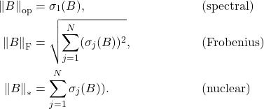
But what do we mean by best approximation? One ingredient we need is a way of measuring how big the discrepancy between two matrices is. Let’s define a measure of the size of a matrix which we will call ‘s norm, which we denote as . If is a matrix and is a low-rank approximation to it, then is a good approximation to if the norm is small. There might be many different ways of measuring the size of the error, but we have to insist on a couple of properties on our norm for it to really define a sensible measure of size. For instance if the norm of a matrix is , then the norm of should be . A list of the properties we require a norm to have are listed on the Wikipedia page for norms. We shall also insist on one more property for our norm: the norm should be unitarily invariant.¹¹Note that every unitarily invariant norm is a special type of vector norm (called a symmetric gauge function) evaluated on the singular values of the matrix. What this means is the norm of a matrix remains the same if it is multiplied on the left or right by an orthogonal matrix. This property is reasonable since multiplication by orthogonal matrices geometrically represents a rotation or reflection¹²This is not true in dimensions higher than 2, but it gives the right intuition that orthogonal matrices preserve distances. which preserves distances between points, so it makes sense that we should demand that the size of a matrix as measured by our norm does not change by such multiplications. Two important and popular matrix norms satisfy the unitarily invariant property: the Frobenius norm and the spectral (or operator 2-) norm , which measures the largest singular value.¹³Both the Frobenius and spectral norms are examples of an important subclass of unitarily invariant norms called Schatten norms. Another example of a Schatten norm, important in matrix completion, is the nuclear norm (sum of the singular values).

With this preliminary out of the way, the Eckart–Young theorem states that the truncated singular value decomposition of truncated to rank is the closest of all rank- matrices when distances are measured using any unitarily invariant norm . If we let denote the -truncated singular value decomposition of , then the Eckart–Young theorem states that

(5)  

Less precisely, the -truncated singular value decomposition is the best rank- approximation to a matrix.

Let’s unpack the Eckart–Young theorem using the spectral and Frobenius norms. In this context, a brief calculation and the Eckart–Young theorem proves that for any rank- matrix , we have

(6)  

where are the singular values of . This bound is quite intuitive. The error in low-rank approximation will be “small” when we measure the error in the spectral norm when each singular value we zero out is “small”. When we measure error in the Frobenius norm, the error in low-rank approximation is “small” when all of the singular values we zero out are “small” in aggregate when squared and added together.

The Eckart–Young theorem shows that possessing a good low-rank approximation is equivalent to the singular values rapidly decaying.¹⁴At least when measured in unitarily invariant norms. A surprising result shows that even the identity matrix, whose singular values are all equal to one, has good low-rank approximations in the maximum entrywise absolute value norm; see, e.g., Theorem 1.0 in this article. If a matrix does not have nice singular value decay, no good low-rank approximation exists, computed by the -truncated SVD or otherwise.

Why Are So Many Matrices (Approximately) Low-rank?

As we’ve seen, we can perform computations with low-rank matrices represented using rank factorizations much faster than general matrices. But all of this would be a moot point if low-rank matrices rarely occurred in practice. But in fact precisely the opposite is true: Approximately low-rank matrices occur all the time in practice.

Sometimes, exact low-rank matrices appear for algebraic reasons. For instance, when we perform one step Gaussian elimination to compute an factorization, the lower right portion of the eliminated matrix, the so-called Schur complement, is a rank-one update to the original matrix. In such cases, a rank- matrix might appear in a computation when one performs steps of some algebraic process: The appearance of low-rank matrices in such cases is unsurprising.

However, often, matrices appearing in applications are (approximately) low-rank for analytic reasons instead. Consider the weather example from the start again. One might reasonably model the temperature on Earth as a smooth function of position and time . If we then let denote the position on Earth of station and the time representing the th day of a given year, then the entries of the matrix are given by . As discussed in my article on smoothness and degree of approximation, a smooth function function of one variable can be excellently approximated by, say, a polynomial of low degree. Analogously, a smooth function depending on two arguments, such as our function , can be excellently be approximated by a separable expansion of rank :

(7)  

Similar to functions of a single variable, the degree to which a function can to be approximated by a separable function of small rank depends on the degree smoothness of the function . Assuming the function is quite smooth, then can be approximated has a separable expansion of small rank . This leads immediately to a low-rank approximation to the matrix given by the rank factorization

(8)  

Thus, in the context of our weather example, we see that the data matrix can be expected to be low-rank under the reasonable-sounding assumption that the temperature depends smoothly on space and time.

What does this mean in general? Let’s speak informally. Suppose that the th entries of a matrix are samples from a smooth function for points and . Then we can expect that will be approximately low-rank. From a computational point of view, we don’t need to know a separable expansion for the function or even the form of the function itself: If the smooth function exists and is sampled from it, then is approximately low-rank and we can find a low-rank approximation for using the truncated singular value decomposition.¹⁵Note here an important subtlety. A more technically precise version of what we’ve stated here is that: if depending on inputs and is sufficiently smooth for in the product of compact regions and , then an matrix with and will be low-rank in the sense that it can be approximated to accuracy by a rank- matrix where grows slowly as and increase and decreases. Note that, phrased this way, the low-rank property of is asymptotic in the size and and the accuracy . If is not smooth on the entirety of the domain or the size of the domains and grow with and , these asymptotic results may no longer hold. And if and are small enough or is large enough, may not be well approximated by a matrix of small rank. Only when there are enough rows and columns will meaningful savings from low-rank approximation be possible.

This “smooth function” explanation for the prevalence of low-rank matrices is the reason for the appearance of low-rank matrices in fast multipole method-type fast algorithms in computational physics and has been proposed¹⁶This article considers piecewise analytic functions rather than smooth functions; the principle is more-or-less the same. as a general explanation for the prevalence of low-rank matrices in data science.

(Another explanation for low-rank structure for highly structured matrices like Hankel, Toeplitz, and Cauchy matrices¹⁷Computations with these matrices can often also be accelerated with other approaches than low-rank structure; see my post on the fast Fourier transform for a discussion of fast Toeplitz matrix-vector products. which appear in control theory applications has a different explanation involving a certain Sylvester equation; see this lecture for a great explanation.)

Upshot: A matrix is low-rank if it has many fewer linearly independent columns than columns. Such matrices can be efficiently represented using rank-factorizations, which can be used to perform various computations rapidly. Many matrices appearing in applications which are not genuinely low-rank can be well-approximated by low-rank matrices; the best possible such approximation is given by the truncated singular value decomposition. The prevalence of low-rank matrices in diverse application areas can partially be explained by noting that matrices sampled from smooth functions are approximately low-rank.

The famous law of the instrument states that “when all you have is a hammer, every problem looks like a nail.” In general, this tendency is undesirable: most problems in life are not nails and could better be addressed by a more appropriate tool. However, one can also review the law of the instrument in a more positive framing: when presented with a powerful new tool, it is worth checking how many problems it can solve. The fast Fourier transform (FFT) is one of the most important hammers in an applied mathematician’s toolkit. And it has made many seemingly unrelated problems look like nails.

In this article, I want to consider three related questions:

1. What is the FFT—what problem is it solving and how does it solve it fast?
2. How can the ideas behind the FFT be used to solve other problems?
3. How can the FFT be used as a building block in solving a seemingly unrelated problem?

The FFT is widely considered one of the most important numerical algorithms, and as such every sub-community of applied mathematics is inclined to see the most interesting applications of the FFT as those in their particular area. I am unapologetically victim to this tendency myself, and thus will discuss an application of the FFT that I find particularly beautiful and surprising. In particular, this article won’t focus on the manifold applications of the FFT in signal processing, which I think has been far better covered by authors more familiar with that field.

The Discrete Fourier Transform

At its core, the FFT is a fast algorithm to compute complex numbers given real or complex numbers defined by the formula¹The factor of is not universal. It is common to omit the factor in (1) and replace the in Eq. (2) with a . We prefer this convention as it makes the DFT a unitary transformation. When working with Fourier analysis, it is important to choose formulas for the (discrete) Fourier transform and the inverse (discrete) Fourier transform which form a pair in the sense they are inverses of each other.

(1)  

The outputs is called the discrete Fourier transform (DFT) of . The FFT is just one possible algorithm to evaluate the DFT.

The DFT has the following interpretation. Suppose that is a periodic function defined on the integers with period —that is, for every integer . Choose to be the values of given by for . Then, in fact, gives an expression for as a so-called trigonometric polynomial²The name “trigonometric polynomial” is motivated by Euler’s formula which shows that , so indeed the right-hand side of Eq. (2) is indeed a “polynomial” in the “variables” and :

(2)  

This shows that (1) converts function values of a periodic function to coefficients of a trigonometric polynomial representation of , which can be called the Fourier series of . Eq. (2), referred to as the inverse discrete Fourier transform, inverts this, converting coefficients to function values .

Fourier series are an immensely powerful tool in applied mathematics. For example again, if represents a sound wave produced by a chord on a piano, its Fourier coefficients represents the intensity of each pitch comprising the chord. An audio engineer could, for example, compute a Fourier series for a piece of music and zero out Fourier coefficients, thus reducing the amount of data needed to store a piece of music. This idea is indeed part of the way audio compression standards like MP3 work. In addition to many more related applications in signal processing, the Fourier series is also a natural way to solve differential equations, either by pencil and paper or by computer via so-called Fourier spectral methods. As these applications (and more to follow) show, the DFT is a very useful computation to perform. The FFT allows us to perform this calculation fast.

The Fast Fourier Transform

The first observation to make is that Eq. (1) is a linear transformation: if we think of Eq. (1) as describing a transformation , then we have that . Recall the crucial fact from linear algebra that every linear transformation can be represented by a matrix-vector muliplication.³At least in finite dimensions; the story for infinite-dimensional vector spaces is more complicated. In my experience, one of the most effective algorithm design strategies in applied mathematics is, when presented with a linear transformation, to write its matrix down and poke and prod it to see if there are any patterns in the numbers which can be exploited to give a fast algorithm. Let’s try to do this with the DFT.

We have that for some matrix . (We will omit the subscript when its value isn’t particularly important to the discussion.) Let us make the somewhat non-standard choice of describing rows and columns of by zero-indexing, so that the first row of is row and the last is row . Then we have that . Comparing with Eq. (1), we see that . Let us define . Thus, we can write the matrix out as

(3)  

This is a highly structured matrix. The patterns in this matrix are more easily seen for a particular value of . We shall focus on in this discussion, but what will follow will generalize in a straightforward way to any power of two (and in less straightforward ways to arbitrary —we will return to this point at the end).

Instantiating Eq. (3) with (and writing ), we have

(4)  

To fully exploit the patterns in this matrix, we note that represents a clockwise rotation of the complex plane by an eighth of the way around the circle. So, for example is twenty-one eighths of a turn or simply just turns. Thus and more generally . This allows us to simplify as follows:

(5)  

Now notice that, since represents a clockwise rotation of an eighth of the way around the circle, represents a quarter turn of the circle. This fact leads to the surprising observation we can actually find the DFT matrix for hidden inside the DFT matrix for !

To see this, rearrange the columns of to interleave every other column. In matrix language this is represented by right-multiplying with an appropriate⁴In fact, this permutation has a special name: the perfect shuffle. permutation matrix :

(6)  

The top-left sub-block is precisely (up to scaling). In fact, defining the diagonal matrix (called the twiddle factor) and noting that , we have

(7)  

The matrix is entirely built up of simple scalings of the smaller DFT matrix ! This suggests the following decomposition to compute :

(8)  

Here represent the even-indexed entries of and the odd-indexed entries. Thus, we see that we can evaluate by evaluating the two expressions and . We have broken our problem into two smaller problems, which we then recombine into a solution of our original problem.

How then, do we compute the smaller DFTs and ? We just use the same trick again, breaking, for example, the product into further subcomputations and . Performing this process one more time, we need to evaluate expressions of the form , which are simply given by since the matrix is just a matrix whose single entry is .

This procedure is an example of a recursive algorithm: we designed an algorithm which solves a problem by breaking it down into one or more smaller problems, solve each of the smaller problems by using this same algorithm, and then reassemble the solutions of the smaller problems to solve our original problem. Eventually, we will break our problems into such small pieces that they can be solved directly, which is referred to as the base case of our recursion. (In our case, the base case is multiplication by ). Algorithms using this recursion in this way are referred to as divide-and-conquer algorithms.

Let us summarize this recursive procedure we’ve developed. We want to compute the DFT where is a power of two. First, we use the DFT to recursively compute and . Next, we combine these computations to evaluate by the formula

(9)  

This procedure is the famous fast Fourier transform (FFT), whose modern incarnation was presented by Cooley and Tukey in 1965 with lineage that can be traced back to work by Gauss in the early 1800s. There are many variants of the FFT using similar ideas.

Let us see why the FFT is considered “fast” by analyzing its operation count. As is common for divide-and-conquer algorithms, the number of operations for computing using the FFT can be determined by solving a certain recurrence relation. Let be the number of operations required by the FFT. Then the cost of computing consists of

• proportional-to- operations (or operations, in computer science language⁵ refers to big-O notation. Saying an algorithm takes operations is stating that, more or less, the algorithm takes less than some multiple of operations to complete.) to:
  • add, subtract, and scale vectors and
  • multiply by the diagonal matrix and
• two recursive computations of for , each of which requires operations.

This gives us the recurrence relation

(10)  

Solving recurrences is a delicate art in general, but a wide class of recurrences are immediately solved by the flexible master theorem for recurrences. Appealing to this result, we deduce that the FFT requires operations. This is a dramatic improvement of the operations to compute directly using Eq. (1). This dramatic improvement in speed is what makes the FFT “fast”.

Extending the FFT Idea

The FFT is a brilliant algorithm. It exploits the structure of the discrete Fourier transform problem Eq. (1) for dramatically lower operation counts. And as we shall see a taste of, the FFT is useful in a surprisingly broad range of applications. Given the success of the FFT, we are naturally led to the question: can we learn from our success with the FFT to develop fast algorithms for other problems?

I think the FFT speaks to the power of a simple problem-solving strategy for numerical algorithm design⁶As mentioned earlier, the FFT also exemplifies a typical design pattern in general (not necessarily numerical) algorithm design, the divide-and-conquer strategy. In the divide-and-conquer strategy, find a clever way of dividing a problem into multiple subproblems, conquering (solving) each, and then recombining the solutions to the subproblems into a solution of the larger problem. The challenge with such problems is often finding a way of doing the recombination step, which usually relies on some clever insight. Other instances of divide-and-conquer algorithms include merge sort and Karatsuba’s integer multiplication algorithm.: whenever you have a linear transformation, write it as a matrix-vector product; whenever you have a matrix, write it down and see if there are any patterns.⁷Often, rearranging the matrix will be necessary to see any patterns. We often like to present mathematics with each step of a derivation follows almost effortlessly from the last from a firm basis of elegant mathematical intuition. Often, however, noticing patterns by staring at symbols on a page can be more effective than reasoning grounded in intuition. Once the pattern has been discovered, intuition and elegance sometimes will follow quickly behind.

The most natural generalization of the FFT is the fast inverse discrete Fourier transform, providing a fast algorithm to compute the inverse discrete Fourier transform Eq. (2). The inverse FFT is quite an easy generalization of the FFT presented in the past section; it is a good exercise to see if you can mimic the development in the previous section to come up with this generalization yourself. The FFT can also be generalized to other discrete trigonometric transforms and 2D and 3D discrete Fourier transforms.

I want to consider a problem more tangentially related to the FFT, the evaluation of expressions of the form , where is an matrix, is an matrix, is a vector of length , and denotes the Kronecker product. For the unitiated, the Kronecker product of and is a matrix defined as the block matrix

(11)  

We could just form this matrix and compute the matrix-vector product directly, but this takes a hefty operations.⁸Equally or perhaps more problematically, this also takes space. We can do better.

The insight is much the same as with the FFT: scaled copies of the matrix are embedded in . In the FFT, we needed to rearrange the columns of the DFT matrix to see this; for the Kronecker product, this pattern is evident in the natural ordering. To exploit this fact, chunk the vectors and into pieces and of length and respectively so that our matrix vector product can be written as⁹This way of writing this expression is referred to as a conformal partitioning to indicate that one can multiply the block matrices using the ordinary matrix product formula treating the block entries as if they were simple numbers.

(12)  

To compute this product efficiently, we proceed in two steps. First, we compute the products which takes time in total. Next, we compute each component by using the formula

(13)  

which takes a total of operations to compute all the ‘s. This leads to a total operation count of for computing the matrix-vector product , much better than our earlier operation count of .¹⁰There is another way of interpreting this algorithm. If we interpret and as the vectorization of and matrices and , then we have . The algorithm we presented is equivalent to evaluating this matrix triple product in the order . This shows that this algorithm could be further accelerated using Strassen–style fast matrix multiplication algorithms.

While this idea might seem quite far from the FFT, if one applies this idea iteratively, one can use this approach to rapidly evaluate a close cousin of the DFT called the Hadamard-Walsh transform. Using the Kronecker product, the Hadamard-Walsh transform of a vector is defined to be

(14)  

If one applies the Kronecker product trick we developed repeatedly, this gives an algorithm to evaluate the Hadamard-Walsh transform of a vector of length in operations, just like the FFT.

The Hadamard-Walsh transform can be thought of as a generalization of the discrete Fourier transform to Boolean functions, which play an integral role in computer science. The applications of the Hadamard-Walsh transform are numerous and varied, from everything to voting systems to quantum computing. This is really just the tip of the iceberg. The ideas behind the FFT (and related ideas from the fast multipole method) allow for the rapid evaluation of a large number of transformations, some of which are connected by deep and general theories.

Resisting the temptation to delve into these interesting subjects in any more depth, we return to our main idea: when presented with a linear transformation, write it as a matrix-vector product; whenever you have a matrix, write it down and see if there are any patterns. The FFT exploits one such pattern, noticing that (after a reordering) a matrix contains many scaled copies of the same matrix. Rapidly evaluation expressions of the form involves an even simpler application of the same idea. But there are many other patterns that can be exploited: sparsity, (approximate) low rank, off-diagonal blocks approximately of low rank, and displacement structure are other examples. Very often in applied math, our problems have additional structure that can be exploited to solve problems much faster, and sometimes finding that structure is as easy as just trying to look for it.

An Application of the FFT

A discussion of the FFT would be incomplete without exploring at least one reason why you’d want to compute the discrete Fourier transform. To focus our attention, let us consider another linear algebraic calculation which appears to have no relation to the FFT on its face: computing a matrix-vector product with a Toeplitz matrix. A matrix is said to be Toeplitz if it has the following structure:

(15)  

Toeplitz matrices and their relatives appear widely across applications of applied mathematics including control and systems theory, time series, numerical partial differential equations, and signal processing.

We seek to compute the matrix-vector product . Let us by considering a special case of a Toeplitz matrix, a circulant matrix. A circulant matrix has the form

(16)  

By direct computation, the matrix-vector product is given by

(17)  

A surprising and non-obvious fact is that the circulant matrix is diagonalized by the discrete Fourier transform. Specifically, we have where . This gives a fast algorithm to compute in time : compute the DFTs of and and multiply them together entrywise, take the inverse Fourier transform, and scale by .

There is a connection with signal processing and differential equations that may help to shed light on why technique works for those familiar with those areas. In the signal processing context, the matrix-vector product can be interpreted as the discrete convolution of with (see Eq. (17)) which is a natural extension of the convolution of two functions and on the real line. It is an important fact that the Fourier transform of a convolution is the same as multiplication of the Fourier transforms: (up to a possible normalizing constant).¹¹A related identity also holds for the Laplace transform. The fact that the DFT diagonalizes a circulant matrix is just the analog of this fact for the discrete Fourier transform and the discrete convolution.

This fast algorithm for circulant matrix-vector products is already extremely useful. One can naturally reframe the problems of multiplying integers and polynomials as discrete convolutions, which can then be computed rapidly by applying the algorithm for fast circulant matrix-vector products. This video gives a great introduction to the FFT with this as its motivating application.

Let’s summarize where we’re at. We are interested in computing the Toeplitz matrix-vector product . We don’t know how to do this for a general Toeplitz matrix yet, but we can do it for a special Toeplitz matrix called a circulant matrix . By use of the FFT, we can compute the circulant matrix-vector product in operations.

We can now leverage what we’ve done with circulant matrices to accelerate Toeplitz matrix-vector product. The trick is very simple: embedding. We construct a big circulant matrix which contains the Toeplitz matrix as a sub-matrix and then use multiplications by the bigger matrix to compute multiplications by the smaller matrix.

Consider the following circulant matrix, which contains as as defined in Eq. (15) a sub-matrix in its top-left corner:

(18)  

This matrix is hard to write out, but essentially we pad the Toeplitz matrix with extra zeros to embed it into a circulant matrix. The “” vector for this larger circulant matrix is obtained from the parameters of the Toeplitz matrix Eq. (15) by .

Here comes another clever observation: we can choose the number of padding zeros used cleverly to make the size of exactly equal to a power of two. This is useful because it allows us to compute matrix-vector products with the power-of-two FFT described above, which we know is fast.

Finally, let’s close the loop and use fast multiplications with to compute fast multiplications with . We wish to compute the product fast. To do this, vector into a larger vector by padding with zeros to get

(19)  

where we use to denote matrix or vector entries which are immaterial to us. We compute by using our fast algorithm to compute and then discarding everything but the first entries of to obtain . If you’re careful to analyze how much padding we need to make this work, we see that this algorithm also takes only operations. Thus, we’ve completed our goal: we can compute Toeplitz matrix-vector products in a fast operations.

Finally, let us bring this full circle and see a delightfully self-referential use of this algorithm: we can use the FFT-accelerated fast Toeplitz matrix-vector multiply to compute DFT itself. Recall that the FFT algorithm we presented above was particularized to which were powers of . There are natural generalizations of the along the lines of what we did above to more general which are highly composite and possess many small prime factors. But what if we want to evaluate the DFT for which is a large prime?

Recall that the DFT matrix has th entry . We now employ a clever trick. Let be a diagonal matrix with the th entry equal to . Then, defining , we have that , which means is a Toeplitz matrix! (Writing out the matrix entrywise may be helpful to see this.)

Thus, we can compute the DFT for any size by evaluating the DFT as , where the product is computed using the fast Toeplitz matrix-vector product. Since our fast Toeplitz matrix-vector product only requires us to evaluate power-of-two DFTs, this technique allows us to evaluate DFTs of arbitrary size in only operations.

Upshot: The discrete Fourier transform (DFT) is an important computation which occurs all across applied mathematics. The fast Fourier transform (FFT) reduces the operation count of evaluating the DFT of a vector of length to proportional to , down from proportional to for direct evaluation. The FFT is an example of a broader matrix algorithm design strategy of looking for patterns in the numbers in a matrix and exploiting these patterns to reduce computation. The FFT can often have surprising applications, such as allowing for rapid computations with Toeplitz matrices.

My first experience with the numerical solution of partial differential equations (PDEs) was with finite difference methods. I found finite difference methods to be somewhat fiddly: it is quite an exercise in patience to, for example, work out the appropriate fifth-order finite difference approximation to a second order differential operator on an irregularly spaced grid and even more of a pain to prove that the scheme is convergent. I found that I liked the finite element method a lot better¹Finite element methods certainly have their own fiddly-nesses (as anyone who has worked with a serious finite element code can no doubt attest to). as there was a unifying underlying functional analytic theory, Galerkin approximation, which showed how, in a sense, the finite element method computed the best possible approximate solution to the PDE among a family of potential solutions. However, I came to feel later that Galerkin approximation was, in a sense, the more fundamental concept, with the finite element method being one particular instantiation (with spectral methods, boundary element methods, and the conjugate gradient method being others). In this post, I hope to give a general introduction to Galerkin approximation as computing the best possible approximate solution to a problem within a certain finite-dimensional space of possibilities.

Systems of Linear Equations

Let us begin with a linear algebraic example, which is unburdened by some of the technicalities of partial differential equations. Suppose we want to solve a very large system of linear equations , where the matrix is symmetric and positive definite (SPD). Suppose that is where is so large that we don’t even want to store all components of the solution on our computer. What can we possibly do?

One solution is to consider only solutions lying in a subspace of the set of all possible solutions . If this subspace has a basis , then the solution can be represented as and one only has to store the numbers . In general, will not belong to the subspace and we must settle for an approximate solution .

The next step is to convert the system of linear equations into a form which is more amenable to approximate solution on a subspace . Note that the equation encodes different linear equations where is the th row of and is the th element of . Note that the th equation is equivalent to the condition , where is the vector with zeros in all entries except for the th entry which is a one. More generally, by multiplying the equation by an arbitrary test row vector , we get for all . We refer to this as a variational formulation of the linear system of equations . In fact, one can easily show that the variational problem is equivalent to the system of linear equations:

(1)  

Since we are seeking an approximate solution from the subspace , it is only natural that we also restrict our test vectors to lie in the subspace . Thus, we seek an approximate solution to the system of equations as the solution of the variational problem

(2)  

One can relatively easily show this problem possesses a unique solution .²Here is a linear algebraic proof. As we shall see below, the same conclusion will also follow from the general Lax-Milgram theorem. Let be a matrix whose columns form a basis for . Then every can be written as for some . Thus, writing , we have that for every . But this is just a variational formulation of the equation . The matrix is SPD since for since is SPD. Thus has a unique solution . Thus is the unique solution to the variational problem Eq. (2). In what sense is a good approximate solution for ? To answer this question, we need to introduce a special way of measuring the error to an approximate solution to . We define the -inner product of a vector and to be and the associated -norm .³Note that -norm can be seen as a weighted Euclidean norm, where the components of the vector in the direction of the eigenvectors of are scaled by their corresponding eigenvector. Concretely, if where is an eigenvector of with eigenvalue (), then we have . All of the properties satisfied by the familiar Euclidean inner product and norm carry over to the new -inner product and norm (e.g., the Pythagorean theorem). Indeed, for those familiar, one can show satisfies all the axioms for an inner product space.

We shall now show that the error between and its Galerkin approximation is -orthogonal to the space in the sense that for all . This follows from the straightforward calculation, for ,

(3)  

where since solves the variational problem Eq. (1) and since solves the variational problem Eq. (2).

The fact that the error is -orthogonal to can be used to show that is, in a sense, the best approximate solution to in the subspace . First note that, for any approximate solution to , the vector is -orthogonal to . Thus, by the Pythagorean theorem,

(4)  

Thus, the Galerkin approximation is the best approximate solution to in the subspace with respect to the -norm, for every . Thus, if one picks a subspace for which the solution almost lies in ⁴In the sense that is small then will be a good approximate solution to , irrespective of the size of the subspace .

Variational Formulations of Differential Equations

As I hope I’ve conveyed in the previous section, Galerkin approximation is not a technique that only works for finite element methods or even just PDEs. However, differential and integral equations are one of the most important applications of Galerkin approximation since the space of all possible solution to a differential or integral equation is infinite-dimensional: approximation in a finite-dimensional space is absolutely critical. In this section, I want to give a brief introduction to how one can develop variational formulations of differential equations amenable to Galerkin approximation. For simplicity of presentation, I shall focus on a one-dimensional problem which is described by an ordinary differential equation (ODE) boundary value problem. All of this generalized wholesale to partial differential equations in multiple dimensions, though there are some additional technical and notational difficulties (some of which I will address in footnotes). Variational formulation of differential equations is a topic with important technical subtleties which I will end up brushing past. Rigorous references are Chapters 5 and 6 from Evans’ Partial Differential Equations or Chapters 0-2 from Brenner and Scott’s The Mathematical Theory of Finite Element Methods.

As our model problem for which we seek a variational formulation, we will focus on the one-dimensional Poisson equation, which appears in the study of electrostatics, gravitation, diffusion, heat flow, and fluid mechanics. The unknown is a real-valued function on an interval which take to be .⁵In higher dimensions, one can consider an arbitrary domain with, for example, a Lipschitz boundary. We assume Dirichlet boundary conditions that is equal to zero on the boundary .⁶In higher dimensions, one has on the boundary of the region . Poisson’s equations then reads⁷ on and for higher dimensions, where is the Laplacian operator.

(5)  

We wish to develop a variational formulation of this differential equation, similar to how we develop a variational formulation of the linear system of equations in the previous section. To develop our variational formulation, we take inspiration from physics. If represents, say, the temperature at a point , we are never able to measure exactly. Rather, we can measure the temperature in a region around with a thermometer. No matter how carefully we engineer our thermometer, our thermometer tip will have some volume occupying a region in space. The temperature measured by our thermometer will be the average temperature in the region or, more generally, a weighted average where is a weighting function which is zero outside the region . Now let’s use our thermometer to “measure” our differential equation:

(6)  

This integral expression is some kind of variational formulation of our differential equation, as it is an equation involving the solution to our differential equation which must hold for every averaging function . (The precise meaning of every will be forthcoming.) It will benefit us greatly to make this expression more “symmetric” with respect to and . To do this, we shall integrate by parts:⁸Integrating by parts is harder in higher dimensions. My personal advice for integrating by parts in higher dimensions is to remember that integration by parts is ultimately a result of the product rule. As such, to integrate by parts, we first write an expression involving our integrand using the product rule of some differential operator and then integrate by both sides. In this case, notice that . Rearranging and integrating, we see that . We then apply the divergence theorem to the last term to get , where represents an outward facing unit normal to the boundary and represents integration on the surface . If is zero on , we conclude for all nice functions on satisfying on .

(7)  

In particular, if is zero on the boundary , then the second two terms vanish and we’re left with the variational equation

(8)  

Compare the variational formulation of the Poisson equation Eq. (8) to the variational formulation of the system of linear equations in Eq. (1). The solution vector in the differential equation context is a function satisfying the boundary condition of being zero on the boundary . The right-hand side is replaced by a function on the interval . The test vector is replaced by a test function on the interval . The matrix product expression is replaced by the integral . The product is replaced by the integral . As we shall soon see, there is a unifying theory which treats both of these contexts simultaneously.

Before this unifying theory, we must address the question of which functions we will consider in our variational formulation. One can show that all of the calculations we did in this section hold if is a continuously differentiable function on which is zero away from the endpoints and and is a twice continuously differentiable function on . Because of technical functional analytic considerations, we shall actually want to expand the class of functions in our variational formulation to even more functions . Specifically, we shall consider all functions which are (A) square-integrable ( is finite), (B) possess a square integrable derivative⁹More specifically, we only insist that possess a square-integrable weak derivative. ( is finite), and (C) are zero on the boundary. We refer to this class of functions as the Sobolev space .¹⁰The class of functions satisfying (A) and (B) but not necessarily (C) is the Sobolev space . For an arbitrary function in , the existence of a well-defined restriction to the boundary and is actually nontrivial to show, requiring showing the existence of a trace operator. Chapter 5 of Evan’s Partial Differential Equations is a good introduction to Sobolev spaces. The Sobolev spaces and naturally extend to spaces and for an arbitrary domain with a nice boundary.

Now this is where things get really strange. Note that it is possible for a function to satisfy the variational formulation Eq. (8) but for not to satisfy the Poisson equation Eq. (5). A simple example is when possesses a discontinuity (say, for example, a step discontinuity where is and then jumps to ). Then no continuously differentiable will satisfy Eq. (5) at every point in and yet a solution to the variational problem Eq. (8) exists! The variational formulation actually allows us to give a reasonable definition of “solving the differential equation” when a classical solution to does not exist. Our only requirement for the variational problem is that , itself, belongs to the space . A solution to the variational problem Eq. (8) is called a weak solution to the differential equation Eq. (5) because, as we have argued, a weak solution to Eq. (8) need not always solve Eq. (5).¹¹One can show that any classical solution to Eq. (5) solves Eq. (8). Given certain conditions on , one can go the other way, showing that weak solutions are indeed bonafide classical solutions. This is the subject of regularity theory.

The Lax-Milgram Theorem

Let us now build up an abstract language which allows us to use Galerkin approximation both for linear systems of equations and PDEs (as well as other contexts). If one compares the expressions from the linear systems context and from the differential equation context, one recognizes that both these expressions are so-called bilinear forms: they depend on two arguments ( and or and ) and are a linear transformation in each argument independently if the other one is fixed. For example, if one defines one has . Similarly, if one defines , then .

Implicitly swimming in the background is some space of vectors or function which this bilinear form is defined upon. In the linear system of equations context, this space of -dimensional vectors and in the differential context, this space is as defined in the previous section.¹²The connection between vectors and functions is even more natural if one considers a function as a vector of infinite length, with one entry for each real number . Call this space . We shall assume that is a special type of linear space called a Hilbert space, an inner product space (with inner product ) where every Cauchy sequence converges to an element in (in the inner product-induced norm).¹³Note that every inner product space has a unique completion to a Hilbert space. For example, if one considers the space of smooth functions which are zero away from the boundary of with the inner product , the completion is . A natural extension to higher dimensions hold. The Cauchy sequence convergence property, also known as metric completeness, is important because we shall often deal with a sequence of entries which we will need to establish convergence to a vector . (Think of as a sequence of Galerkin approximations to a solution .)

With these formalities, an abstract variational problem takes the form

(9)  

where is a bilinear form on and is a linear form on (a linear map ). There is a beautiful and general theorem called the Lax-Milgram theorem which establishes existence and uniqueness of solutions to a problem like Eq. (9).

Theorem (Lax-Milgram): Let and satisfy the following properties:

1. (Boundedness of ) There exists a constant such that every , .
2. (Coercivity) There exists a positive constant such that for every .
3. (Boundedness of ) There exists a constant such that for every .

Then the variational problem Eq. (9) possesses a unique solution.

For our cases, will also be symmetric for all . While the Lax-Milgram theorem holds without symmetry, let us continue our discussion with this additional symmetry assumption. Note that, taken together, properties (1-2) say that the -inner product, defined as , is no more than so much bigger or smaller than the standard inner product of and .¹⁴That is, one has that the -norm and the -norm are equivalent in the sense that . so the norms and define the same topology.

Let us now see how the Lax-Milgram theorem can apply to our two examples. For a reader who wants a more “big picture” perspective, they can comfortably skip to the next section. For those who want to see Lax-Milgram in action, see the discussion below.

Applying the Lax-Milgram Theorem

Begin with the linear system of equations with with inner product , , and . Note that we have the inequality .¹⁵This is an easy consequence of the Courant-Fischer theorem. More generally, note that, since is symmetric, has an orthonormal basis of eigenvectors with eigenvalues . Then and . The inequalities follow from noting the Parseval relation and noting that is a convex combination of the eigenvalues of . In particular, we have that . Property (1) then follows from the Cauchy-Schwarz inequality applied to the -inner product: . Property (2) is simply the established inequality . Property (3) also follows from the Cauchy-Schwarz inequality: . Thus, by Lax-Milgram, the variational problem for has a unique solution . Note that the linear systems example shows why the coercivity property (2) is necessary. If is positive semi-definite but not positive-definite, then there exists an eigenvector of with eigenvalue . Then for any positive constant and is singular, so the variational formulation of has no solution for some choices of the vector .

Applying the Lax-Milgram theorem to differential equations can require powerful inequalities. In this case, the -inner product is given by , , and . Condition (1) is follows from a application of the Cauchy-Schwarz inequality for integrals:¹⁶ In higher dimensions, we need even more Cauchy-Schwarz! First, we note that the absolute value of integral is less than the integral of absolute value . Second, we apply the Cauchy-Schwarz inequality for the vectors and to get where, e.g., is the Euclidean norm of the vector . This gives . Next, we apply the Cauchy-Schwarz inequality for integrals to get . Finally, we note that and thus obtain . This is the desired inequality with constant one.

(10)  

Let’s go line-by-line. First, we note that the absolute value of integral is less than the integral of absolute value. Next, we apply the Cauchy-Schwarz inequality for integrals. Finally, we note that . This establishes Property (1) with constant . As we already see one third of the way into verifying the hypotheses of Lax-Milgram, establishing these inequalities can require several steps. Ultimately, however, strong knowledge of just a core few inequalities (e.g. Cauchy-Schwarz) may be all that’s needed.

Proving coercivity (Property (2)) actually requires a very special inequality, Poincaré’s inequality.¹⁷In higher dimensions, Poincaré’s inequality takes the form for a constant depending only on the domain . In it’s simplest incarnation, the inequality states that there exists a constant such that, for all functions ,¹⁸A simple proof of Poincaré’s inequality for continuously differentiable with goes as follows. Note that, by the fundamental theorem of calculus, . Applying the Cauchy-Schwarz inequality for integrals gives since . Thus for all integrating over gives . This proves Poincaré’s inequality with the constant .

(11)  

With this inequality in tow, property (2) follows after another lengthy string of inequalities:¹⁹The same estimate holds in higher dimensions, with the appropriate generalization of Poincaré’s inequality.

(12)  

For Property (3) to hold, the function must be square-integrable. With this hypothesis, Property (3) is much easier than Properties (1-2) and we leave it as an exercise for the interested reader (or to a footnote²⁰The proof is similar in one dimension or higher dimensions, so we state it for arbitrary domain for brevity. By Cauchy-Schwarz, we have that . for the uninterested reader).

This may seem like a lot of work, but the result we have achieved is stunning. We have proven (modulo a lot of omitted details) that the Poisson equation has a unique weak solution as long as is square-integrable!²¹And in the footnotes, we have upgraded this proof to existence of a unique weak solution to the Poisson equation on a domain . What is remarkable about this proof is that it uses the Lax-Milgram theorem and some inequalities alone: no specialized knowledge about the physics underlying the Poisson equation were necessary. Going through the details of Lax-Milgram has been a somewhat lengthy affair for an introductory post, but hopefully this discussion has illuminated the power of functional analytic tools (like Lax-Milgram) in studying differential equations. Now, with a healthy dose of theory in hand, let us return to Galerkin approximation.

General Galerkin Approximation

With our general theory set up, Galerkin approximation for general variational problem is the same as it was for a system of linear equations. First, we pick an approximation space which is a subspace of . We then have the Galerkin variational problem

(13)  

Provided and satisfy the conditions of the Lax-Milgram theorem, there is a unique solution to the problem Eq. (13). Moreover, the special property of Galerkin approximation holds: the error is -orthogonal to the subspace . Consequently, is te best approximate solution to the variational problem Eq. (9) in the -norm. To see the -orthogonality, we have that, for any ,

(14)  

where we use the variational equation Eq. (9) for and Eq. (13) for . Note the similarities with Eq. (3). Thus, using the Pythagorean theorem for the -norm, for any other approximation solution , we have²²Compare Eq. (4).

(15)  

Put simply, is the best approximation to in the -norm.²³Using the fact the norms and are equivalent in virtue of Properties (1-2), one can also show that is within a constant factor of the best approximation in the norm . This is known as Céa’s Lemma.

Galerkin approximation is powerful because it allows us to approximate an infinite-dimensional problem by a finite-dimensional one. If we let be a basis for the space , then the approximate solution can be represented as . Since form a basis of , to check that the Galerkin variational problem Eq. (13) holds for all it is sufficient to check that it holds for .²⁴For an arbitrary can be written as , so . Thus, plugging in and into Eq. (13), we get (using bilinearity of )

(16)  

If we define and , then this gives us a matrix equation for the unknowns parametrizing . Thus, we can compute our Galerkin approximation by solving a linear system of equations.

We’ve covered a lot of ground so let’s summarize. Galerkin approximation is a technique which allows us to approximately solve a large- or infinite-dimensional problem by searching for an approximate solution in a smaller finite-dimensional space of our choosing. This Galerkin approximation is the best approximate solution to our original problem in the -norm. By choosing a basis for our approximation space , we reduce the problem of computing a Galerkin approximation to a linear system of equations.

Design of a Galerkin approximation scheme for a variational problem thus boils down to choosing the approximation space and a basis . Picking to be a space of piecewise polynomial functions (splines) gives the finite element method. Picking to be a space spanned by a collection of trigonometric functions gives a Fourier spectral method. One can use a space spanned by wavelets as well. The Galerkin framework is extremely general: give it a subspace and it will give you a linear system of equations to solve to give you the best approximate solution in .

Two design considerations factor into the choice of space and basis . First, one wants to pick a space , where the solution almost lies in. This is the rationale behind spectral methods. Smooth functions are very well-approximated by short truncated Fourier expansions, so, if the solution is smooth, spectral methods will converge very quickly. Finite element methods, which often use low-order piecewise polynomial functions, converge much more slowly to a smooth . The second design consideration one wants to consider is the ease of solving the system resulting from the Galerkin approximation. If the basis function are local in the sense that most pairs of basis functions and aren’t nonzero at the same point (more formally, and have disjoint supports for most and ), the system will be sparse and thus usually much easier to solve. Traditional spectral methods usually result in a harder-to-solve dense linear systems of equations.²⁵There are clever ways of making spectral methods which lead to sparse matrices. Conversely, if one uses high-order piecewise polynomials in a finite element approximation, one can get convergence properties similar to a spectral method. These are called spectral element methods. It should be noted that both spectral and finite element methods lead to ill-conditioned matrices , making integral equation-based approaches preferable if one needs high-accuracy.²⁶For example, only one researcher using a finite-element method was able to meet Trefethen’s challenge to solve the Poisson equation to eight digits of accuracy on an L-shaped domain (see Section 6 of this paper). Getting that solution required using a finite-element method of order 15! Integral equations, themselves, are often solved using Galerkin approximation, leading to so-called boundary element methods.

Upshot: Galerkin approximation is a powerful and extremely flexible methodology for approximately solving large- or infinite-dimensional problems by finding the best approximate solution in a smaller finite-dimensional subspace. To use a Galerkin approximation, one must convert their problem to a variational formulation and pick a basis for the approximation space. After doing this, computing the Galerkin approximation reduces down to solving a system of linear equations with dimension equal to the dimension of the approximation space.

Sparse matrices are an indispensable tool for anyone in computational science. I expect there are a very large number of simulation programs written in scientific research across the country which could be faster by ten to a hundred fold at least just by using sparse matrices! In this post, we’ll give a brief overview what a sparse matrix is and how we can use them to solve problems fast.

A matrix is sparse if most of its entries are zero. There is no precise threshold for what “most” means; Kolda suggests that a matrix have at least 90% of its entries be zero for it to be considered sparse. The number of nonzero entries in a sparse matrix is denoted by . A matrix that is not sparse is said to be dense.

Sparse matrices are truly everywhere. They occur in finite difference, finite element, and finite volume discretizations of partial differential equations. They occur in power systems. They occur in signal processing. They occur in social networks. They occur in intermediate stages in computations with dense rank-structured matrices. They occur in data analysis (along with their higher-order tensor cousins).

Why are sparse matrices so common? In a word, locality. If the th entry of a matrix is nonzero, then this means that row and column are related in some way to each other according to the the matrix . In many situations, a “thing” is only related to a handful of other “things”; in heat diffusion, for example, the temperature at a point may only depend on the temperatures of nearby points. Thus, if such a locality assumption holds, every row will only have a small number of nonzero entries and the matrix overall will be sparse.

Storing and Multiplying Sparse Matrices

A sparse matrix can be stored efficiently by only storing its nonzero entries, along with the row and column in which these entries occur. By doing this, a sparse matrix can be stored in space rather than the standard for an matrix .¹Here, refers to big-O notation. For the efficiency of many algorithms, it will be very beneficial to store the entries row-by-row or column-by-column using compressed sparse row and column (CSR and CSC) formats; most established scientific programming software environments support sparse matrices stored in one or both of these formats. For efficiency, it is best to enumerate all of the nonzero entries for the entire sparse matrix and then form the sparse matrix using a compressed format all at once. Adding additional entries one at a time to a sparse matrix in a compressed format requires reshuffling the entire data structure for each new nonzero entry.

There exist straightforward algorithms to multiply a sparse matrix stored in a compressed format with a vector to compute the product . Initialize the vector to zero and iterate over the nonzero entries of , each time adding to . It is easy to see this algorithm runs in time.²More precisely, this algorithm takes time since it requires operations to initialize the vector even if has no nonzero entries. We shall ignore this subtlety in the remainder of this article and assume that , which is true of most sparse matrices occurring in practice The fact that sparse matrix-vector products can be computed quickly makes so-called Krylov subspace iterative methods popular for solving linear algebraic problems involving sparse matrices, as these techniques only interact with the matrix by computing matrix-vector products (or matrix-tranpose-vector products ).

Lest the reader think that every operation with a sparse matrix is necessarily fast, the product of two sparse matrices and need not be sparse and the time complexity need not be . A counterexample is

(1)  

for . We have that but

(2)  

which has nonzero elements and requires operations to compute. However, if one does the multiplication in the other order, one has and the multiplication can be done in operations. Thus, some sparse matrices can be multiplied fast and others can’t. This phenomena of different speeds for different sparse matrices is very much also true for solving sparse linear systems of equations.

Solving Sparse Linear Systems

The question of how to solve a sparse system of linear equations where is sparse is a very deep problems with fascinating connections to graph theory. For this article, we shall concern ourselves with so-called sparse direct methods, which solve by means of computing a factorization of the sparse matrix . These methods produce an exact solution to the system if all computations are performed exactly and are generally considered more robust than inexact and iterative methods. As we shall see, there are fundamental limits on the speed of certain sparse direct methods, which make iterative methods very appealing for some problems.

Note from the outset that our presentation will be on illustrating the big ideas rather than presenting the careful step-by-step details needed to actually code a sparse direct method yourself. An excellent reference for the latter is Tim Davis’ wonderful book Direct Methods for Sparse Linear Systems.

Let us begin by reviewing how factorization works for general matrices. Suppose that the entry of is nonzero. Then, factorization proceeds by subtracting scaled multiples of the first row from the other rows to zero out the first column. If one keeps track of these scaling, then one can write this process as a matrix factorization, which we may demonstrate pictorially as

(3)  

Here, ‘s denote nonzero entries and blanks denote zero entries. We then repeat the process on the submatrix in the bottom right (the so-called Schur complement). Continuing in this way, we eventually end up with a complete factorization

(4)  

In the case that is symmetric positive definite (SPD), one has that for a diagonal matrix consisting of the entries on . This factorization is a Cholesky factorization of .³Often, the Cholesky factorization is written as for or for . These different forms all contain the same basic information, so we shall stick with the formulation in this post. For general non-SPD matrices, one needs to incorporate partial pivoting for Gaussian elimination to produce accurate results.⁴See the excellent monograph Accuracy and Stability of Numerical Algorithms for a comprehensive treatment of this topic.

Let’s try the same procedure for a sparse matrix. Consider a sparse matrix with the following sparsity pattern:

(5)  

When we eliminate the entry, we get the following factorization:

(6)  

Note that the Schur complement has new additional nonzero entries (marked with a ) not in the original sparse matrix . The Schur complement of is denser than was; there are new fill-in entries. The worst-case scenario for fill-in is the arrowhead matrix:

(7)  

After one step of Gaussian elimination, we went from a matrix with nonzeros to a fully dense Schur complement! However, the arrowhead matrix also demonstrates a promising strategy. Simply construct a permutation matrix which reorders the first entry to be the last⁵For instance, the circular shift permutation . and then perform Gaussian elimination on the symmetrically permuted matrix instead. In fact, the entire factorization can be computed without fill-in:

(8)  

This example shows the tremendous importance of reordering of the rows and columns when computing a sparse factorization.

The Best Reordering

As mentioned above, when computing an factorization of a dense matrix, one generally has to reorder the rows (and/or columns) of the matrix to compute the solution accurately. Thus, when computing the factorization of a sparse matrix, one has to balance the need to reorder for accuracy and to reorder to reduce fill-in. For these reasons, for the remainder of this post, we shall focus on computing Cholesky factorizations of SPD sparse matrices, where reordering for accuracy is not necessary.⁶For ill-conditioned and positive semi-definite matrices, one may want to reorder a Cholesky factorization so the result is rank-revealing. This review article has a good discussion of pivoted Cholesky factorization. For most applications, one can successfully compute an accurate Cholesky factorization without any specific accuracy-focused reordering strategy. Since we want the matrix to remain SPD, we must restrict ourselves to symmetric reordering strategies where is reordered to where is a permutation matrix.

Our question is deceptively simple: what reordering produces the least fill-in? In matrix language, what permutation minimizes where is the Cholesky factorization of ?

Note that, assuming no entries in the Gaussian elimination process exactly cancel, then the Cholesky factorization depends only on the sparsity pattern of (the locations of the zeros and nonzeros) and not on the actual numeric values of ‘s entries. This sparsity structure is naturally represented by a graph whose nodes are the indices with an edge between if, and only if, .

Now let’s see what happens when we do Gaussian elimination from a graph point-of-view. When we eliminate the entry from matrix, this results in all nodes of the graph adjacent to becoming connected to each other.⁷Graph theoretically, we add a clique containing the nodes adjacent to

This shows why the arrowhead example is so bad. By eliminating the a vertex connected to every node in the graph, the eliminated graph becomes a complete graph.

Reordering the matrix corresponds to choosing in what order the vertices of the graph are eliminated. Choosing the elimination order is then a puzzle game; eliminate all the vertices of the graph in the order that produces the fewest fill-in edges (shown red).⁸This “graph game” formulation of sparse Gaussian elimination is based on how I learned it from John Gilbert. His slides are an excellent resource for all things sparse matrices!

Finding the best elimination ordering for a sparse matrix (graph) is a good news/bad news situation. For the good news, many graphs possess a perfect elimination ordering, in which no fill-in is produced at all. There is a simple algorithm to determine whether a graph (sparse matrix) possesses a perfect elimination ordering and if so, what it is.⁹The algorithm is basically just a breadth-first search. Some important classes of graphs can be eliminated perfectly (for instance, trees). More generally, the class of all graphs which can be eliminated perfectly is precisely the set of chordal graphs, which are well-studied in graph theory.

Now for the bad news. The problem of finding the best elimination ordering (with the least fill-in) for a graph is NP-Hard. This means, assuming the widely conjectured result that , that finding the best elimination ordering would be a hard computational problem than the worst-case complexity for doing Gaussian elimination in any ordering! One should not be too pessimistic about this result, however, since (assuming ) all it says is that there exists no polynomial time algorithm guaranteed to produce the absolutely best possible elimination ordering when presented with any graph (sparse matrix). If one is willing to give up on any one of the bolded statements, further progress may be possible. For instance, there exists several good heuristics, which find reasonably good elimination orderings for graphs (sparse matrices) in linear (or nearly linear) time.

Can Sparse Matrices be Eliminated in Linear Time?

Let us think about the best reordering question in a different way. So far, we have asked the question “Can we find the best ordering for a sparse matrix?” But another question is equally important: “How efficiently can we solve a sparse matrix, even with the best possible ordering?”

One might optimistically hope that every sparse matrix possesses an elimination ordering such that its Cholesky factorization can be computed in linear time (in the number of nonzeros), meaning that the amount of time needed to solve is proportional to the amount of data needed to store the sparse matrix .

When one tests a proposition like this, one should consider the extreme cases. If the matrix is dense, then it requires operations to do Gaussian elimination,¹⁰This is neglecting the possibility of acceleration by Strassen–type fast matrix multiplication algorithms. For simplicity, we shall ignore these fast multiplication techniques for the remainder of this post and assume dense can be solved no faster than operations. but only has nonzero entries. Thus, our proposition cannot hold in unmodified form.

An even more concerning counterexample is given by a matrix whose graph is a 2D grid graph.

Sparse matrices with this sparsity pattern (or related ones) appear all the time in discretized partial differential equations in two dimensions. Moreover, they are truly sparse, only having nonzero entries. Unforunately, no linear time elimination ordering exists. We have the following theorem:

Theorem: For any elimination ordering for a sparse matrix with being a 2D grid graph, in any elimination ordering, the Cholesky factorization requires operations and satisfies .¹¹Big-Omega notation is a cousin of Big-O notation. One should read as “ is no less than a constant multiple of , asymptotically”.

The proof is contained in Theorem 10 and 11 (and the ensuing paragraph) of classic paper by Lipton, Rose, and Tarjan. Natural generalizations to -dimensional grid graphs give bounds of time and for . In particular, for 2D finite difference and finite element discretizations, sparse Cholesky factorization takes operations and produces a Cholesky factor with in the best possible ordering. In 3D, sparse Cholesky factorization takes operations and produces a Cholesky factor with in the best possible ordering.

Fortunately, at least these complexity bounds are attainable: there is an ordering which produces a sparse Cholesky factorization with requiring operations and with nonzero entries in the Cholesky factor.¹²Big-Theta notation just means if and One such asymptotically optimal ordering is the nested dissection ordering, one of the heuristics alluded to in the previous section. The nested dissection ordering proceeds as follows:

1. Find a separator consisting of a small number of vertices in the graph such that when is removed from , is broken into a small number of edge-disjoint and roughly evenly sized pieces .¹³In particular, is the disjoint union and there are no edges between and for .
2. Recursively use nested dissection to eliminate each component individually.
3. Eliminate in any order.

For example, for the 2D grid graph, if we choose to be a cross through the center of the 2D grid graph, we have a separator of size dividing the graph into roughly pieces.

Let us give a brief analysis of this nested dissection ordering. First, consider the sparsity of the Cholesky factor . Let denote the number of nonzeros in for an elimination of the 2D grid graph using the nested dissection ordering. Then step 2 of nested dissection requires us to recursively eliminate four 2D grid graphs. After doing this, for step 3, all of the vertices of the separator might be connected to each other, so the separator graph will potentially have as many as edges, which result in nonzero entries in . Thus, combining the fill-in from both steps, we get

(9)  

Solving this recurrence using the master theorem for recurrences gives . If one instead wants the time required to compute the Cholesky factorization, note that for step 3, in the worst case, all of the vertices of the separator might be connected to each other, leading to a dense matrix. Since a matrix requires , we get the recurrence

(10)  

which solves to .

Conclusions

As we’ve seen, sparse direct methods (as exemplified here by sparse Cholesky) possess fundamental scalability challenges for solving large problems. For the important class of 2D and 3D discretized partial differential equations, the time to solve scales like and , respectively. For truly large-scale problems, these limitations may be prohibitive for using such methods.

This really is the beginning of the story, not the end for sparse matrices however. The scalability challenges for classical sparse direct methods has spawned many exciting different approaches, each of which combats the scalability challenges of sparse direct methods for a different class of sparse matrices in a different way.

Upshot: Sparse matrices occur everywhere in applied mathematics, and many operations on them can be done very fast. However, the speed of computing an factorization of a sparse matrix depends significantly on the arrangement of its nonzero entries. Many sparse matrices can be factored quickly, but some require significant time to factor in any reordering.

At its core, computational mathematics is about representing the infinite by the finite. Even attempting to store a single arbitrary real number requires an infinite amount of memory to store its infinitely many potentially nonrepeating digits.¹It is a well-known result that a real number has a repeating decimal expansion if, and only if, it is rational. When dealing with problems in calculus, however, the problem is even more severe as we want to compute with functions on the real line. In effect, a function is an uncountably long list of real numbers, one for each value of the function’s domain. We certainly cannot store an infinite list of numbers with infinitely many digits on a finite computer!

Thus, our only hope to compute with functions is to devise some sort of finite representation for them. The most natural representation is to describe function by a list of real numbers (and then store approximations of these numbers on our computer). For instance, we may approximate the function by a polynomial of degree and then store the coefficients . From this list of numbers, we then can reconstitute an approximate version of the function. For instance, in our polynomial example, our approximate version of the function is just . Naturally, there is a tradeoff between the length of our list of numbers and how accurate our approximation is. This post is about that tradeoff.

The big picture idea is that the “smoother” a function is, the easier it will be to approximate it with a small number of parameters. Informally, we have the following rule of thumb: if a function on a one-dimensional domain possesses nice derivatives, then can be approximated by a -parameter approximation with error decaying at least as fast as . This basic result appears in many variants in approximation theory with different precise definitions of the term “ nice derivatives” and “-parameter approximation”. Let us work out the details of the approximation problem in one concrete setting using Fourier series.

Approximation by Fourier Series

Consider a complex-valued and -period function defined on the real line. (Note that, by a standard transformation, there are close connections between approximation of -periodic functions on the whole real line and functions defined on a compact interval .²Specifically, suppose that is a function defined on . Then define a function on by . This linear rescaling of the domain is very simple and easy to understand. Now define a -periodic function on by . There are very close connections between approximation of and . For example, Fourier cosine expansions of are equivalent to Chebyshev polynomial expansions of . For more on this subject, Trefethen’s Approximation Theory and Approximation Practice is an excellent reference.) If is square-integrable, then possesses a Fourier expansion

(1)  

The infinite series converges in the sense, meaning that , where is the truncated Fourier series and is norm .³One may show with considerable analysis that Fourier series converges in others senses, for example almost everywhere convergence. We also have the Plancherel theorem, which states that

(2)  

Note that the convergence of the Fourier series is fundamentally a statement about approximation. The fact that the Fourier series converges means that the truncated Fourier series of terms acts as an arbitrarily close approximate of (measured with the norm). However, the number of terms we need to store might be quite large if a large value of is needed for to be small. However, as we shall soon see, if the function is “smooth”, will be small for even moderate values of .

Smoothness

Often, in analysis, we refer to a function as smooth when it possesses derivatives of all orders. In one dimension, this means that the th derivative exists for every integer . In this post, we shall speak of smoothness as a more graded notion: loosely, a function is smoother than a function if possesses more derivatives than or the magnitude of ‘s derivatives are smaller. This conception of smoothness accords more with the plain-English definition of smoothness: the graph of a very mildly varying function with a discontinuity in its 33rd derivative looks much smoother to the human eye than the graph of a highly oscillatory and jagged function that nonetheless possesses derivatives of all orders.⁴One might refer to the precise concept of possessing derivatives of all orders as smoothness.

For a function defined in terms of a Fourier series, it is natural to compute its derivative by formally differentiating the Fourier series term-by-term:

(3)  

This formal Fourier series converges if, and only if, the norm of this putative derivative , as computed with the Plancherel theorem, is finite: . This “derivative” may not be a derivative of in the classical sense. For instance, using this definition, the absolute value function possesses a derivative for and for . For the derivative of to exist in the sense of Eq. (3), need not be differentiable at every point, but it must define a square-integrable functions at the points where it is differentiable. We shall call the derivative as given by Eq. (3) to be a weak derivative of .

If a function has square-integrable weak derivatives for , then we say that belongs to the Sobolev space . The Sobolev space is equipped with the norm

(4)  

The Sobolev norm is a quantitative measure of qualitative smoothness. The smaller the Sobolev norm of , the smaller the derivatives of are. As we will see, we can use this to bound the approximation error.

Smoothness and Degree of Approximation

If is approximated by , the error of approximation is given by

(5)  

Suppose that (that is, has square integrable derivatives). Then we may deduce the inequality

(6)  

The first “” follows from the fact that for . This very important result is a precise instantiation of our rule of thumb from earlier: if possesses nice (i.e. square-integrable) derivatives, then the () approximation error for an -term Fourier approximation decays at least as fast as .

Higher Dimensions

The results for one dimension can easily be extended to consider functions defined on -dimensional space which are -periodic in every argument.⁵e.g. for every For physics-based scientific simulation, we are often interested in or , but for more modern problems in data science, we might be interested in very large dimensions .

Letting denote the set of all -tuples of integers, one can show that one has the -dimensional Fourier series

(7)  

Here, we denote to be the Euclidean inner product of the -dimensional vectors and , . A natural generalization of the Plancherel theorem holds as well. Let denote the maximum of . Then, we have the truncated Fourier series . Using the same calculations from the previous section, we deduce a very similar approximation property

(8)  

There’s a pretty big catch though. The approximate function possesses terms! In order to include each of the first Fourier modes in each of dimensions, the number of terms in our Fourier approximation must grow exponentially in ! In particular, the approximation error satisfies a bound

(9)  

where is a constant depending only on and .

This is the so-called curse of dimensionality: to approximate a function in dimensions, we need exponentially many terms in the dimension . In higher-dimensions, our rule of thumb needs to be modified: if a function on a -dimensional domain possesses nice derivatives, then can be approximated by a -parameter approximation with error decaying at least as fast as .

The Theory of Nonlinear Widths: The Speed Limit of Approximation Theory

So far, we have shown that if one approximates a function on a -dimensional space by truncating its Fourier series to terms, the approximation error decays at least as fast as . Can we do better than this, particularly in high-dimensions where the error decay can be very slow if ?

One must be careful about how one phrases this question. Suppose I ask “what is the best way of approximating a function “? A subversive answer is that we may approximate by a single-parameter approximation of the form with ! Consequently, there is a one-parameter approximation procedure that approximates every function perfectly. The problem with this one-parameter approximation is obvious: the one-parameter approximation is terrible at approximating most functions different than . Thus, the question “what is the best way of approximating a particular function?” is ill-posed. We must instead ask the question “what is the best way of approximating an entire class of functions?” For us, the class of functions shall be those which are sufficiently smooth: specifically, we shall consider the class of functions whose Sobolev norm satisfies a bound . Call this class .

As outlined at the beginning, an approximation procedure usually begins by taking the function and writing down a list of numbers . Then, from this list of numbers we reconstruct a function which serves as an approximation to . Formally, this can be viewed as a mathematical function which takes to a tuple followed by a function which takes and outputs a continuous -periodic function .

(10)  

Remarkably, there is a mathematical theory which gives sharp bounds on the expressive power of any approximation procedure of this type. This theory of nonlinear widths serves as a sort of speed limit in approximation theory: no method of approximation can be any better than the theory of nonlinear widths says it can. The statement is somewhat technical, and we advise the reader to look up a precise statement of the result before using it any serious work. Roughly, the theory of nonlinear widths states that for any continuous approximation procedure⁶That is, an approximation procedure for which is a continuous function where is equipped with the topology defined by the norm . that is able to approximate every function in with approximation error no more than , the number of parameters must be at least some constant multiple of . Equivalently, the worst-case approximation error for a function in with an parameter continuous approximation is at least some multiple of .

In particular, the theory of nonlinear widths states that the approximation property of truncated Fourier series are as good as any method for approximating functions in the class , as they exactly meet the “speed limit” given by the theory of nonlinear widths. Thus, approximating using truncated Fourier series is, in a certain very precise sense, as good as any other approximation technique you can think of in approximating arbitrary functions from : splines, rational functions, wavelets, and artificial neural networks must follow the same speed limit. Make no mistake, these other methods have definite advantages, but degree of approximation for the class is not one of them. Also, note that the theory of nonlinear widths shows that the curse of dimensionality is not merely an artifact of Fourier series; it affects all high-dimensional approximation techniques.

For the interested reader, see the following footnotes for two important ways one may perform approximations better than the theory of nonlinear widths within the scope of its rules.⁷The theory of nonlinear widths holds for continuous methods of approximation. This means that discontinuous approximation procedures may circumvent its bounds. Indeed, such discontinuous approximation procedures exist using probabilistic techniques. These methods are of questionable use in practice since discontinuous approximation procedures, by their nature, are extremely sensitive to the perturbations which are ubiquitous in performing computations on computers.⁸The theory of nonlinear widths holds for means of approximating the entire class . More efficient methods may exist for meaningful subclasses of . For instance, Mhaskar and Poggio show that for functions satisfying a compositional property, that they can effectively be approximated by multilayer artificial neural networks.

Upshot: The smoother a function is, the better it can be approximated. Specifically, one can approximate a function on dimensions with nice derivatives with approximation error decaying with rate at least . In the case of -periodic functions, such an approximation can easily be obtained by truncating the function’s Fourier series. This error decay rate is the best one can hope for to approximate all functions of this type.

Given the diversity of applications of mathematics, the field of applied mathematics lacks a universally accepted set of core concepts which most experts would agree all self-proclaimed applied mathematicians should know. Further, much mathematical writing is very carefully written, and many important ideas can be obscured by precisely worded theorems or buried several steps into a long proof.

In this series of blog posts, I hope to share my personal experience with some techniques in applied mathematics which I’ve seen pop up many times. My goal is to isolate a single particularly interesting idea and provide a simple explanation of how it works and why it can be useful. In doing this, I hope to collect my own thoughts on these topics and write an introduction to these ideas of the sort I wish I had when I was first learning this material.

Given my fondness for linear algebra, I felt an appropriate first topic for this series would be the Schur Complement. Given matrices , , , and of sizes , , , and with invertible, the Schur complement is defined to be the matrix .

The Schur complement naturally arises in block Gaussian elimination. In vanilla Gaussian elimination, one begins by using the -entry of a matrix to “zero out” its column. Block Gaussian elimination extends this idea by using the submatrix occupying the top-left portion of a matrix to “zero out” all of the first columns together. Formally, given the matrix , one can check by carrying out the multiplication that the following factorization holds:

(1)  

Here, we let denote an identity matrix of size and the zero matrix. Here, we use the notation of block (or partitioned) matrices where, in this case, a matrix is written out as a “block” matrix whose entries themselves are matrices of the appropriate size that all matrices occurring in one block row (or column) have the same number of rows (or columns). Two block matrices which are blocked in a compatible way can be multiplied just like two regular matrices can be multiplied, taking care of the noncommutativity of matrix multiplication.

The Schur complement naturally in the expression for the inverse of . One can verify that for a block triangular matrix , we have the inverse formula

(2)  

(This can be verified by carrying out the block multiplication for the proposed formula for and verifying that one obtains the identity matrix.) A similar formula holds for block lower triangular matrices. From here, we can deduce a formula for the inverse of . Let be the Schur complement. Then

(3)  

This remarkable formula gives the inverse of in terms of , , , and . In particular, the -block entry of  is simply just the inverse of the Schur complement.

Here, we have seen that if one starts with a large matrix and performs block Gaussian elimination, one ends up with a smaller matrix called the Schur complement whose inverse appears in inverse of the original matrix. Very often, however, it benefits us to run this trick in reverse: we begin with a small matrix, which we recognize to be the Schur complement of a larger matrix. In general, dealing with a larger matrix is more difficult than a smaller one, but very often this larger matrix will have special properties which allow us to more efficiently compute the inverse of the original matrix.

One beautiful application of this idea is the Sherman-Morrison-Woodbury matrix identity. Suppose we want to find the inverse of the matrix . Notice that this is the Schur complement of the matrix , which is the same after reordering.¹Specifically, move the switch the first rows with the last rows and do the same with the columns. This defines a permutation matrix such that . Alternately, and perhaps more cleanly, one may define two Schur complements of the block matrix : one by “eliminating “, , and the other by “eliminating “, . Following the calculation in Eq. (3), just like the inverse of the Schur complement appears in the entry of , the inverse of the alternate Schur complement can be shown to appear in the entry of . Thus, comparing with Eq. (3), we deduce the Sherman-Morrison-Woodbury matrix identity:

(4)  

To see how this formula can be useful in practice, suppose that we have a fast way of solving the system linear equations . Perhaps is a simple matrix like a diagonal matrix or we have already pre-computed an factorization for . Consider the problem of solving the rank-one updated problem . Using the Sherman-Morrison-Woodbury identity with , , and , we have that

(5)  

Careful observation of this formula shows how we can compute (solving ) by only solving two linear systems for and for .²Further economies can be saved if one has already previously computed , which may be the case in many applications.

Here’s another variant of the same idea. Suppose we want solve the linear system of equation where is a diagonal matrix. Then we can immediately write down the lifted system of linear equations

(6)  

One can easily see that is the Schur complement of the matrix (with respect to the block). This system of linear equations is sparse in the sense that most of its entries are zero and can be efficiently solved by sparse Gaussian elimination, for which there exists high quality software. Easy generalizations of this idea can be used to effectively solve many “sparse + low-rank” problems.

Another example of the power of the Schur complement are in least-squares problems. Consider the problem of minimizing , where is a matrix with full column rank and is the Euclidean norm of a vector . It is well known that the solution satisfies the normal equations . However, if the matrix is even moderately ill-conditioned, the matrix will be much more ill-conditioned (the condition number will be squared), leading to a loss of accuracy. It is for this reason that it is preferable to solve the least-squares problem with factorization. However, if factorization isn’t available, we can use the Schur complement trick instead. Notice that is the Schur complement of the matrix . Thus, we can solve the normal equations by instead solving the (potentially, see footnote) much better-conditioned system³More precisely, one should scale the identity in the block of this system to be on the order of the size of the entries in . The conditioning is sensitive to the scaling. If one selects a scale to be proportional to the smallest singular value  of and constructs , then one can show that the two-norm condition number of no more than twice that of . If one picks to be roughly equal to the largest singular value , then the two-norm condition number of is roughly the square of the condition number of . The accuracy of this approach may be less sensitive to the scaling parameter than this condition number analysis suggests.

(7)  

In addition to (often) being much better-conditioned, this system is also highly interpretable. Multiplying out the first block row gives the equation which simplifies to . The unknown is nothing but the least-squares residual. The second block row gives , which encodes the condition that the residual is orthogonal to the range of the matrix . Thus, by lifting the normal equations to a large system of equations by means of the Schur complement trick, one derives an interpretable way of solving the least-squares problem by solving a linear system of equations, no factorization or ill-conditioned normal equations needed.

The Schur complement trick continues to have use in areas of more contemporary interest. For example, the Schur complement trick plays a central role in the theory of sequentially semiseparable matrices which is a precursor to many recent developments in rank-structured linear solvers. I have used the Schur complement trick myself several times in my work on graph-induced rank-structures.

Upshot: The Schur complement appears naturally when one does (block) Gaussian elimination on a matrix. One can also run this process in reverse: if one recognizes a matrix expression (involving a product of matrices potentially added to another matrix) as being a Schur complement of a larger matrix , one can often get considerable dividends by writing this larger matrix down. Examples include a proof of the Sherman-Morrison-Woodbury matrix identity (see Eqs. (3-4)), techniques for solving a low-rank update of a linear system of equations (see Eqs. (5-6)), and a stable way of solving least-squares problems without the need to use factorization (see Eq. (7)).

Additional resource: My classmate Chris Yeh has a great introduction to the Schur complements focusing more on positive semidefinite and rank-deficient matrices.

Edits: This blog post was edited to clarify the conditioning of the augmented linear system Eq. (7) and to include a reference to Chris’ post on Schur complements.