Note to Self: How Accurate is Sketch and Solve?

February 12, 2025 by Ethan N. Epperly Leave a comment

Suppose we’re interested in solving an overdetermined linear least-squares problem

(1) $x = \operatorname*{argmin}_{x \in \real^n} \norm{b-Ax}, \quad A \in \real^{m\times n}, \quad b \in \real^m.$

Sketch-and-solve is a popular method for getting a fast, approximate solution to (1). Let $S \in \real^{d\times m}$ be a sketching matrix for $\onebytwo{A}{b}$ of distortion $\eta$ (see these previous posts of mine for a refresher on sketching if needed):

(2) $(1-\eta)\norm{y} \le \norm{Sy} \le (1+\eta)\norm{y} \quad \text{for every } y \in \operatorname{range}(\onebytwo{A}{b}).$

The sketch-and-solve solution to (1) is given by

(3) $\hat{x} = \operatorname*{argmin}_{\hat{x}\in\real^n} \norm{Sb-(SA)\hat{x}}.$

How small is the residual $\norm{b-A\hat{x}}$ of the sketch-and-solve solution? Here’s a one bound:

Proposition 1 (Sketch-and-solve, $1+\order(\eta)$ bound). The sketch-and-solve solution (3) satisfies the bound
$\norm{b-A\hat{x}} \le \frac{1+\eta}{1-\eta} \cdot \norm{b-Ax} = (1 + 2\eta + \order(\eta^2))\norm{b-Ax}.$

Let’s prove this bound. The residual $b-A\hat{x}$ is in the range of $\onebytwo{A}{b}$ . Therefore, by (2),

$(1-\eta) \norm{b-A\hat{x}} \le \norm{S(b-A\hat{x})}.$

Rearranging gives

$\norm{b-A\hat{x}} \le \frac{1}{1-\eta}\norm{S(b-A\hat{x})}.$

By the optimality of the sketch-and-solve solution (3), $\norm{S(b-A\hat{x})}$ is minimized for the value $\hat{x}$ . Thus, its value can only increase by replacing $\hat{x}$ by $x$ :

$\norm{b-A\hat{x}} \le \frac{1}{1-\eta}\norm{S(b-A\hat{x})}\le \frac{1}{1-\eta}\norm{S(b-Ax)}.$

Invoke property (2) a final time to obtain

(4) $\norm{b-A\hat{x}} \le \frac{1}{1-\eta}\norm{S(b-A\hat{x})}\le \frac{1}{1-\eta}\norm{S(b-Ax)}\le \frac{1+\eta}{1-\eta}\cdot \norm{b-Ax}.$

We’ve completed the proof of Proposition 1. In fact, were we to want to write the proof concisely, equation (4) represents a single-line proof of Proposition 1.

The conclusion of Proposition 1 appears to be that the residual norm $\norm{b-A\hat{x}}$ may be a factor $1+\order(\eta^1)$ larger than the minimal least-squares residual $\norm{b-Ax}$ . Interestingly, this conclusion is not sharp. In fact, the residual for sketch-and-solve can only be at most $1+\order(\eta^2)$ larger than optimal. This fact has been known at least since the work of Drineas, Mahoney, Muthukrishnan, and Sarlós (2007). The note of Larsen and Kolda (2022) provides a nice summary of Drineas et al.’s argument. My goal in this post is to simplify this argument even further, making it as elementary as possible.

Notation

To make our lives easier, we’ll begin by defining some notation. Let

(5) $A = UC \quad \text{for } U\in\real^{m\times n}, \: B \in \real^{n\times n}$

be any factorization of $A$ into a matrix $U$ with orthonormal columns and a square nonsingular matrix $C$ . Such a factorization can be computed using a QR or polar decomposition. Let

$r = b-Ax$

denote the optimal least-squares residual. We will have occasion to scale $r$ so that it is a unit vector

$\overline{r} = \frac{r}{\norm{r}}.$

Note that the optimality condition for the least-squares problem (1) is that the residual $r$ is orthogonal to $\operatorname{range}(A)$ . Consequently,

(6) $\onebytwo{U}{\overline{r}} \quad \text{is an orthonormal basis for } \operatorname{range}(\onebytwo{A}{b}).$

Sketching the basis

As saw in (6), the matrix $\onebytwo{U}{\overline{r}}$ is an orthonormal basis for $\operatorname{range}(\onebytwo{A}{b})$ . To get a sharper analysis of sketch-and-solve, we will need the following result, which shows that $S\onebytwo{U}{\overline{r}}$ is an “almost orthonormal basis”.

Lemma 2 (Sketching the basis): The matrix $S\onebytwo{U}{\overline{r}}$ has nearly orthonormal columns in the sense that

(7) $\sigma_{\rm min}(S\onebytwo{U}{\overline{r}}) \ge 1-\eta, \quad \sigma_{\rm max}(S\onebytwo{U}{\overline{r}}) \le 1+\eta.$

Consequently,

(8) $\norm{\onebytwo{U}{\overline{r}}^\top S^\top S\onebytwo{U}{\overline{r}} - I} \le 2\eta+\eta^2.$

This result is a pretty direct reformulation of the sketching property (2). By the variational characterization of the minimum singular value, we have

$\sigma_{\rm min}(S\onebytwo{U}{\overline{r}}) = \min_{\norm{z}=1} \norm{S\onebytwo{U}{\overline{r}}z}.$

The vector $\onebytwo{U}{\overline{r}}z$ is in the range of $\onebytwo{A}{b}$ . Thus, by (2),

$\sigma_{\rm min}(S\onebytwo{U}{\overline{r}}) = \min_{\norm{z}=1} \norm{S\onebytwo{U}{\overline{r}}z} \ge (1-\eta) \min_{\norm{z}=1} \norm{\onebytwo{U}{\overline{r}}z} = 1-\eta.$

For the last equality, we used the fact that $\onebytwo{U}{\overline{r}}$ has orthonormal columns and thus

$\norm{\onebytwo{U}{\overline{r}}z} = \norm{z} \quad \text{for every } z \in \real^{n+1}.$

This proves the first inequality in (7). The second inequality follows along similar lines.

For a tall matrix $F$ , the eigenvalues of $F^\top F$ are equal to the squared singular values of $F$ . Applying this result to $F = \onebytwo{U}{\overline{r}}$ gives

$(1-\eta)^2 \le \lambda_{\rm min}(\onebytwo{U}{\overline{r}}^\top S^\top S\onebytwo{U}{\overline{r}}) \le \lambda_{\rm max}(\onebytwo{U}{\overline{r}}^\top S^\top S\onebytwo{U}{\overline{r}}) \le (1+\eta)^2.$

Subtracting the identity matrix shifts all the eigenvalues down by $1$ :

$-2\eta+\eta^2 \le \lambda_{\rm min}(\onebytwo{U}{\overline{r}}^\top S^\top S\onebytwo{U}{\overline{r}}-I) \le \lambda_{\rm max}(\onebytwo{U}{\overline{r}}^\top S^\top S\onebytwo{U}{\overline{r}}-I) \le 2\eta+\eta^2.$

The spectral norm is equal to the largest eigenvalue in absolute value. Thus

$\norm{\onebytwo{U}{\overline{r}}^\top S^\top S\onebytwo{U}{\overline{r}}-I} \le \max(2\eta+\eta^2,-(-2\eta+\eta^2)) = 2\eta+\eta^2.$

This proves (8).

Sketch-and-Solve: Better Analysis

With Lemma 2 in hand, we are ready to state and prove our main result:

Theorem 3 (Sketch-and-solve, $1+\order(\eta^2)$ bound). The sketch-and-solve solution (3) satisfies the bound
(9) $\norm{b-A\hat{x}}^2 \le \left(1 + \frac{(2\eta+\eta^2)^2}{(1-\eta)^4}\right) \norm{b-Ax}^2 \le \left(1 + \frac{9\eta^2}{(1-\eta)^4}\right)\norm{b-Ax}^2.$
As a consequence,
(10) $\norm{b-A\hat{x}}^2 \le (1+4\eta^2+\order(\eta^3)) \norm{b-Ax}^2$
and
(11) $\norm{b-A\hat{x}} \le (1+2\eta^2+\order(\eta^3)) \norm{b-Ax}.$

Let’s prove Theorem 3. Begin by decomposing the sketch-and-solve residual $b - A\hat{x}$ :

$b - A\hat{x} = b - Ax + Ax - A\hat{x} = r + A(\hat{x}-x).$

The residual $r$ is orthogonal to the range of $A$ . Thus, by the Pythagorean theorem,

(12) $\norm{b-A\hat{x}}^2 = \norm{r}^2 + \norm{A(\hat{x}-x)}^2.$

To bound $\norm{A(\hat{x}-x)}^2$ , it will help us to have a more convenient formula for $\hat{x}-x$ . To this end, reparametrize the sketch-and-solve least-squares problem as an optimization problem over the error $e \coloneqq \hat{x} - x$ :

$\hat{x} = \operatorname*{argmin}_{\hat{x}\in\real^n} \norm{S(b - Ax)-SA(\hat{x}-x)} \implies \hat{x} - x = \operatorname*{argmin}_{e\in\real^n} \norm{Sr - SAe}.$

Applying the normal equations to this least-squares problem, we get

$\hat{x} - x = (A^\top S^\top SA)^{-1} A^\top S^\top Sr.$

Now, invoke the factorization (5):

$\hat{x} - x = C^{-1} (U^\top S^\top SU)^{-1} U^\top S^\top Sr.$

Thus,

$A(\hat{x} - x) = U(U^\top S^\top SU)^{-1} U^\top S^\top Sr.$

Taking norms and using the definition $r = \norm{r} \cdot \overline{r}$ , we obtain

(13) $\norm{A(\hat{x} - x)} \le \norm{(U^\top S^\top S U)^{-1}} \cdot \norm{U^\top S^\top S \overline{r}} \cdot \norm{r}.$

We now work to bound the two factors in (10). The matrix $SU$ is a submatrix of $S\onebytwo{U}{\overline{r}}$ . Thus, by (7),

$\sigma_{\rm min}(SU) \ge \sigma_{\rm min}(S\onebytwo{U}{\overline{r}}) \ge 1-\eta.$

Consequently,

$\norm{(U^\top S^\top S U)^{-1}} = \sigma_{\rm min}^2(SU) \le \frac{1}{(1-\eta)^2}.$

The matrix $U^\top S^\top S\overline{r}$ is a submatrix of $\onebytwo{U}{\overline{r}}S^\top S\onebytwo{U}{\overline{r}} - I$ . Thus, by (8),

$\norm{U^\top S^\top S \overline{r}} \le \norm{\onebytwo{U}{\overline{r}}S^\top S\onebytwo{U}{\overline{r}} - I}\le 2\eta + \eta^2.$

Substituting the two previous displays into (13) yields

$\norm{A(\hat{x} - x)} \le \frac{2\eta+\eta^2}{(1-\eta)^2} \cdot \norm{r}.$

Plugging this display into (12) proves (9). Equations (10) and (11) follow from (9) and a Taylor series expansion. This proves Theorem 3.

Can We Do Better?

In the limit $\eta \to 0$ , Theorem 3 identifies the correct $1+\order(\eta^2)$ scaling for sketch-and-solve, consistent both with numerical experiments, exact computations for Gaussian embeddings, and lower bounds for solving least-squares problems by row subselection. However, comparing results for Gaussian embeddings shows there may be room for improvement. Here is an informal statement of the Gaussian results:

Informal Theorem 4 (Gaussian sketch-and-solve): Appropriately scaled, a $d\times m$ Gaussian matrix is an $\eta$ -sketching matrix provided $d\approx n/\eta^2$ . The expected least-squares residual is
(14) $\expect \norm{b - A\hat{x}}^2 \approx \left(1 + \frac{\eta^2}{(1+\eta)(1-\eta)}\right) \norm{b - Ax}^2.$

See this post of mine for a formal version of this result, its proof, and a discussion of the history of this result. We see that the bound (9) for general embeddings takes the form $1 + \order((1-\eta)^{-4})$ in the limit $\eta\to 1$ , whereas the bound (14) for Gaussian embeddings scales like $1 + \order((1-\eta)^{-1})$ . We leave it as a conjecture/open problem whether there is an improved argument for general subspace embeddings:

Conjecture 5 (Sketch-and-solve, large $\eta$ ): The sketch-and-solve solution (3) satisfies the bound
$\norm{b-A\hat{x}}^2 \le \left(1 + \frac{C\eta^2}{1-\eta}\right)\norm{b-Ax}^2$
for an absolute constant $C > 0$ .

Notes: For another proof demonstrating the correction $\order(\eta^2)$ scaling for a different type of dimensionality reduction (leverage score sampling), check out this article by Raphael Meyer.

My Favorite Proof of the Cauchy–Schwarz Inequality

December 10, 2024 by Ethan N. Epperly 2 Comments

The Cauchy–Schwarz inequality has many proofs. Here is my favorite, taken from Chapter 3 of The Schur complement and its applications; the book is edited by Fuzhen Zhang, and this chapter was contributed by him as well. Let $x,y \in \real^n$ be vectors, assemble the matrix $B = \onebytwo{x}{y}$ , and form the Gram matrix

$A = B^\top B = \onebytwo{x}{y}^\top \onebytwo{x}{y} = \twobytwo{\norm{x}^2}{y^\top x}{x^\top y}{\norm{y}^2}.$

Since $A$ is a Gram matrix, it is positive semidefinite. Therefore, its determinant is nonnegative:

$\det(A) = \norm{x}^2\norm{y}^2 - |x^\top y|^2 \ge 0.$

Rearrange to obtain the Cauchy–Schwarz inequality

$|x^\top y| \le \norm{x}\norm{y}.$

Equality occurs if and only if $A$ is a rank-one matrix, which occurs if and only if $x$ and $y$ are scalar multiples.

I like this proof because it is perhaps the simplest example of the (block) matrix technique for proving inequalities. Using this technique, one proves inequalities about scalars (or matrices) by embedding them in a clever way into a (larger) matrix. Here is another example of the matrix technique, adapted from the proof of Theorem 12.9 of these lecture notes by Joel Tropp. Jensen’s inequality is a far-reaching and very useful inequality in probability theory. Here is one special case of the inequality.

Proposition (Jensen’s inequality for the inverse): Let $x_1,\ldots,x_n$ be strictly positive numbers. Then the inverse of their average is no bigger than the average of their inverses:
$\left( \frac{1}{n} \sum_{i=1}^n x_i \right)^{-1} \le \frac{1}{n} \sum_{i=1}^n \frac{1}{x_i}.$

To prove this result, embed each $x_i$ into a $2\times 2$ positive semidefinite matrix $\twobytwo{x_i}{1}{1}{1/x_i}$ . Taking the average of all such matrices, we observe that

$A = \twobytwo{\frac{1}{n} \sum_{i=1}^n x_i}{1}{1}{\frac{1}{n} \sum_{i=1}^n \frac{1}{x_i}}$

is positive semidefinite as well. Thus, its determinant is nonnegative:

$\det(A) = \left(\frac{1}{n} \sum_{i=1}^n x_i\right) \left(\frac{1}{n} \sum_{i=1}^n \frac{1}{x_i}\right) - 1 \ge 0.$

Rearrange to obtain

$\left( \frac{1}{n} \sum_{i=1}^n x_i \right)^{-1} \le \frac{1}{n} \sum_{i=1}^n \frac{1}{x_i}.$

Remarkably, we have proven a purely scalar inequality by appeals to matrix theory.

The matrix technique for proving inequalities is very powerful. Check out Chapter 3 of The Schur complement and its applications for many more examples.

If you like this blog and want another way to follow it, I am starting newsletter:

Low-Rank Approximation Toolbox: The Gram Correspondence

December 7, 2024 by Ethan N. Epperly Leave a comment

I am delighted to share that my paper Randomly pivoted Cholesky: Randomly pivoted Cholesky: Practical approximation of a kernel matrix with few entry evaluations, joint with Yifan Chen, Joel Tropp, and Robert Webber, has been published online in Communications on Pure and Applied Mathematics. To celebrate this occasion, I want to share one of my favorite tricks in the design of low-rank approximation algorithms, which I will call the Gram correspondence.

Projection Approximation and Nyström Approximation

When we construct a low-rank approximation to a matrix, the type of approximation we use is typically dictated by the size and properties of the matrix. For a rectangular matrix $B \in \real^{M\times N}$ , one of the standard techniques is the standard randomized SVD algorithm:

Generate a Gaussian random matrix $\Omega \in \real^{N\times k}$ .
Form the product $Y = B\Omega$ .
Compute an (economy-size) QR decomposition $Y = QR$ .
Evaluate the SVD $Q^\top B = \tilde{U} \Sigma V^\top$ .
Output the low-rank approximation $\hat{B} = U\Sigma V^\top$ for $U = Q\tilde{U}$ .

Succinctly, the output of the randomized SVD is given by the formula $\hat{B} = \Pi_{B\Omega} B$ , where $\Pi_F$ denotes the orthogonal projector onto the column span of a matrix $F$ . This motivates the general definition:

Definition (projection approximation): Given a test matrix $\Omega \in \real^{N\times k}$ , the projection approximation to the matrix $B$ is $\hat{B} = \Pi_{B\Omega} B$ .

The class of projection approximations is much richer than merely the approximation constructed by the standard randomized SVD. Indeed, low-rank approximations computed by randomized subspace iteration, randomized block Krylov iteration, column-pivoted QR decompositions, etc. all fit under the umbrella of projection approximations.

Many matrices in applications have additional structure such as symmetry or sparsity, and it can be valuable to make use of low-rank approximations that take advantage of those properties. An especially important type of structure is positive semidefiniteness. For our purposes, a positive semidefinite matrix $A \in \real^{N\times N}$ is one that is symmetric and possesses nonnegative eigenvalues, and we will use abbreviate “positive semidefinite” as “psd”. Psd matrices arise in applications as covariance matrices, kernel matrices, and as discretizations of certain differential and integral operators. Further, any rectangular matrix $B \in \real^{M\times N}$ gives rise to its psd Gram matrix $A = B^\top B$ ; we will have much more to say about Gram matrices below.

To compute a low-rank approximation to a psd matrix, the preferred format as usually the Nyström approximation:

Definition (Nyström approximation): Given a test matrix $\Omega \in \real^{N\times k}$ , the Nyström approximation is¹
$\hat{A} \coloneqq (A\Omega) (\Omega^\top A \Omega)^{-1}(A\Omega)^\top.$

As discussed in a previous post, the general class of Nyström approximations includes many useful specializations depending on how the matrix $\Omega$ is selected.

The Gram Correspondence

The Gram correspondence is a connection between projection approximation and Nyström approximation:

The Gram correspondence: Let $B\in\real^{M\times N}$ be any rectangular matrix and consider the Gram matrix $A = B^\top B$ . Fix a test matrix $\Omega$ , and define the Nyström approximation $\hat{A} = A\langle \Omega\rangle$ to $A$ and the projection approximation $\hat{B} = \Pi_{B\Omega}B$ to $B$ . Then
$\hat{A} = \smash{\hat{B}}^\top \hat{B}.$
That is, the Gram matrix $\hat{B}^\top\hat{B}$ of the projection approximation $\hat{B}\approx B$ is the Nyström approximation $\hat{A} \approx A$ .

As we will see, this correspondence has many implications:

Special cases. The correspondence contains several important facts as special cases. Examples include the equivalence between the randomized SVD and single-pass Nyström approximation and the equivalence of (partial) column-pivoted QR factorization and (partial) pivoted Cholesky decomposition.
Algorithm design. Since Nyström approximation and projection approximations are closely related, one can often interconvert algorithms for one type of approximation into the other. These conversions can lead one to discover new algorithms. We will provide a historical answer with the discovery of randomly pivoted Cholesky.
Error bounds. The Gram correspondence is immensely helpful in the analysis of algorithms, as it makes error bounds for projection approximations and Nyström approximations easily derivable from each other.

For those interested, we give a short proof of the Gram correspondence below.

Proof of Gram correspondence

The Gram correspondence is straightforward to derive, so let’s do so before moving on. Because $\Pi_{B\Omega}$ is a projection matrix, it satisfies $\Pi_{B\Omega}^2 = \Pi_{B\Omega}$ . Thus,

$\hat{B}^\top \hat{B} = B^\top \Pi_{B\Omega}^2B = B^\top \Pi_{B\Omega}B.$

The projector $\Pi_F$ has the formula $F (F^\top F)^{-1} F^\top$ . Using this formula, we obtain

$\hat{B}^\top \hat{B} = B^\top B\Omega (\Omega^\top B^\top B \Omega)^{-1} \Omega^\top B^\top B.$

This is precisely the formula for the Nyström approximation $(B^\top B)\langle \Omega\rangle$ , confirming the Gram correspondence.

Aside: Gram Square Roots

Before we go forward, let me highlight a point of potential conclusion and introduce some helpful terminology. When thinking about algorithms for a psd matrix $A$ , it will often to be helpful to conjure a matrix $B$ for which $A = B^\top B$ . Given a psd matrix $A$ , there is always a matrix $B$ for which $A = B^\top B$ , but this $B$ is not unique. Indeed, if $A = B^\top B$ , then we have the infinite family of decompositions $A = (UB)^\top (UB)$ generated by every matrix $U$ with orthonormal columns. This motivates the following definition:

Definition (Gram square root): A matrix $B$ is a Gram square root for $A$ if $A = B^\top B$ .

A Gram square root $B$ for $A$ need not be a square root in the traditional sense that $B^2 = A$ . Indeed, a Gram square root $B$ can be rectangular, so $B^2$ need not even be defined.² Using the Gram square root terminology, the Gram correspondence can be written more succinctly:

Gram correspondence (concise): If $B$ is any Gram square root of $A$ , then the projection approximation $\hat{B} = \Pi_{B\Omega}B$ is a Gram square root of the Nyström approximation $\hat{A} = A\langle \Omega \rangle$ .

Examples of the Gram Correspondence

Before going further, let us see a couple of explicit examples of the Gram correspondence.

Randomized SVD and Single-Pass Nyström Approximation

The canonical example of the Gram correspondence is the equivalence of the randomized SVD algorithm and the single-pass Nyström approximation. Let $B$ be a Gram square root for a psd matrix $A$ . The randomized SVD of $B$ is given by the following steps, which we saw in the introduction:

Generate a Gaussian random matrix $\Omega \in \real^{N\times k}$ .
Form the product $Y = B\Omega$ .
Compute a QR decomposition $Y = QR$ .
Evaluate the SVD $Q^\top B = \tilde{U} \Sigma V^\top$ .
Output the low-rank approximation $\hat{B} = U\Sigma V^\top$ for $U = Q\tilde{U}$ .

Now, imagine taking the same Gaussian matrix $\Omega$ from the randomized SVD, and use it to compute the Nyström approximation $\hat{A} = A\langle \Omega\rangle$ . Notice that this Nyström approximation can be computed in a single pass over the matrix $A$ . Namely, use a single pass over $A$ to compute $Y=A\Omega$ and use following formula:³

$\hat{A} = Y (\Omega^\top Y)^{-1} Y^\top.$

For this reason, we call $\hat{A}$ the single-pass Nyström approximation.

The Gram correspondence tells us that the randomized SVD and single-pass Nyström approximation are closely related, in the sense that $\hat{A} = \hat{B}^\top \hat{B}$ . The randomized SVD approximation $\hat{B}$ is a Gram square root of the single-pass Nyström approximation $\hat{A}$ .

Column-Pivoted QR Factorization and Pivoted Cholesky Decomposition

A more surprising consequence of the Gram correspondence is the connection between low-rank approximations produced by partial column-pivoted QR factorization of a rectangular matrix $B$ and a partial pivoted Cholesky decomposition of $A$ . Let’s begin by describing these two approximation methods.

Let’s begin with pivoted partial Cholesky decomposition. Let $A \in \real^{N\times N}$ be a psd matrix, and initialize the zero approximation $\hat{A} \gets 0$ . For $i=1,2,\ldots,k$ , perform the following steps:

Choose a column index $1 \le s_i \le N$ . These indices are referred to as pivot indices or, more simply, pivots.
Update the low-rank approximation
$\hat{A} \gets \hat{A} + \frac{A(:,s_i)A(s_i,:)}{A(s_i,s_i)}.$
Update the matrix
$A \gets A - \frac{A(:,s_i)A(s_i,:)}{A(s_i,s_i)}.$

Here, we are using MATLAB notation to index the matrix $A$ . The output of this procedure is

$\hat{A} = A(:,S) A(S,S)^{-1} A(S,:),$

where $S = \{s_1,\ldots,s_k\}$ . This type of low-rank approximation is known as a column Nyström approximation and is a special case of the general Nyström approximation with test matrix $\Omega = I(:,S)$ equal to a subset of columns of the identity matrix $I$ . For an explanation of why this procedure is called a “pivoted partial Cholesky decomposition” and the relation to the usual notion of Cholesky decomposition, see this previous post of mine.

Given the Gram correspondence, we expect that this pivoted partial Cholesky procedure for computing a Nyström approximation to a psd matrix $A$ should have an analog for computing a projection approximation to a rectangular matrix $B$ . This analog is given by the partial column-pivoted QR factorization, which produces a low-rank approximation according as follows. Let $B \in \real^{M\times N}$ be a psd matrix, and initialize the zero approximation $\hat{B} \gets 0$ . For $i=1,2,\ldots,k$ , perform the following steps:

Choose a pivot index $1 \le s_i \le N$ .
Update the low-rank approximation by adding the projection of $B$ onto the selected column: $\hat{B} \gets \hat{B} + B(:,s_i) (B(:,s_i)^\top B) / \norm{B(:,s_i)}^2$ .
Update the matrix by removing the projection of $B$ onto the selected column: $B \gets B - B(:,s_i) (B(:,s_i)^\top B) / \norm{B(:,s_i)}^2$ .

The output of this procedure is the column projection approximation $\Pi_{B(:,S)} B$ , which is an example of the general projection approximation with $\Omega = I(:,S)$ .⁴

The pivoted partial Cholesky and QR factorizations are very traditional ways of computing a low-rank approximation in numerical linear algebra. The Gram correspondence tells us immediately that these two approaches are closely related:

Let $B$ be a Gram square root of $A$ . Compute a column projection approximation $\hat{B}$ to $B$ using a partially column-pivoted QR factorization with pivots $s_1,\ldots,s_k$ , and compute a column Nyström approximation $\hat{A}$ to $A$ using a partial pivoted Cholesky decomposition with the same set of pivots $s_1,\ldots,s_k$ . Then $\hat{B}^\top \hat{B} = \hat{A}$ .

I find this remarkable: the equivalence of the randomized SVD and single-pass randomized Nyström approximation and the equivalence of (partial pivoted) Cholesky and QR factorizations are both consequences of the same general principle, the Gram correspondence.

Using the Gram Correspondence to Discover Algorithms

The Gram correspondence is more than just an interesting way of connecting existing types of low-rank approximations: It can be used to discover new algorithms. We can illustrate this with an example, the randomly pivoted Cholesky algorithm.

Background: The Randomly Pivoted QR Algorithm

In 2006, Deshpande, Rademacher, Vempala, and Wang discovered an algorithm that they called adaptive sampling for computing a projection approximation to a rectangular matrix $B \in \real^{M\times N}$ . Beginning from the trivial initial approximation $\hat{B} \gets 0$ , algorithm proceeds as follows for $i=1,2,\ldots,k$ :

Choose a column index $1 \le s_i \le N$ randomly according to the squared column norm distribution:
$\prob\{s_i = j\} = \frac{\norm{B(:,j)}^2}{\norm{B}_{\rm F}^2} \quad \text{for } j=1,2,\ldots,k.$
Update the low-rank approximation by adding the projection of $B$ onto the selected column: $\hat{B} \gets \hat{B} + B(:,s_i) (B(:,s_i)^\top B) / \norm{B(:,s_i)}^2$ .
Update the matrix by removing the projection of $B$ onto the selected column: $B \gets B - B(:,s_i) (B(:,s_i)^\top B) / \norm{B(:,s_i)}^2$ .

Given our discussion above, we recognize this as an example of partial column-pivoted QR factorization with a particular randomized procedure for selecting the pivots $s_i$ .⁵ Therefore, it can also be convenient to call this algorithm randomly pivoted QR.

Randomly pivoted QR is a nice algorithm for rectangular low-rank approximation. Each step requires a full pass over the matrix and $\order(MN)$ operations, so the full procedure requires $\order(MNk)$ operations. This makes the cost of the algorithm similar to other methods for rectangular low-rank approximation such as the randomized SVD, but it has the advantage that it computes a column projection approximation.⁶ However, randomly pivoted QR is not a particularly effective algorithm for computing a low-rank approximation to a psd matrix, since—as we shall see—there are faster procedures available.

Following the Gram correspondence, we expect there should be an analog of the randomly pivoted QR algorithm for computing a low-rank approximation of a psd matrix. That algorithm, which we call randomly pivoted Cholesky, is derived from randomly pivoted QR in the following optional section:

Derivation of Randomly Pivoted Cholesky Algorithm

Let $A \in \real^{N\times N}$ be a psd matrix. For conceptual purposes, let us also consider a Gram square root $B\in \real^{M\times N}$ of $A$ ; this matrix $B$ will only be a conceptual device that we will use to help us derive the appropriate algorithm, not something that will be required to run the algorithm itself. Let us now walk through the steps of the randomly pivoted QR algorithm on $B$ , and see how they lead to a randomly pivoted Cholesky algorithm for computing a low-rank approximation to $A$ .

Step 1 of randomly pivoted QR. Randomly pivoted QR begins by drawing a random pivot $s_i$ according to the rule

$\prob\{s_i = j\} = \frac{\norm{B(:,j)}^2}{\norm{B}_{\rm F}^2} \quad \text{for } j=1,2,\ldots,k.$

Since $A = B^\top B$ , we may compute

$\norm{B(:,j)}^2 = B(:,j)^\top B(:,j) = (B^\top B)(j,j) = A(j,j).$

The squared column norms of $B$ are the diagonal entries of the matrix $A$ . Similarly, $\norm{B}_{\rm F}^2 = \tr(A)$ . Therefore, we can write the probability distribution for the random pivot $s_i$ using only the matrix $A$ as

$\prob\{s_i = j\} = \frac{A(j,j)}{\tr A} \quad \text{for } j=1,2,\ldots,N.$

Step 2 of randomly pivoted QR. The randomly pivoted QR update rule is $\hat{B} \gets \hat{B} + B(:,s_i) (B(:,s_i)^\top B) / \norm{B(:,s_i)}^2$ . Therefore, the update rule for $\hat{A} = \hat{B}^\top\hat{B}$ is

$\hat{A} &\gets \left(\hat{B} + \frac{B(:,s_i) (B(:,s_i)^\top B)}{\norm{B(:,s_i)}^2}\right)^\top \left(\hat{B} + \frac{B(:,s_i) (B(:,s_i)^\top B)}{\norm{B(:,s_i)}^2}\right).$

After a short derivation,⁷, this simplifies to the update rule

$\hat{A} \gets \hat{A} +\frac{A(:,s_i)A(s_i,:)}{A(s_i,s_i)}.$

Two remarkable things have happened. First, we have obtained an update rule for $\hat{A}$ that depends only on the psd matrices $\hat{A}$ and $A$ , and all occurences of the Gram square roots $\hat{B}$ and $B$ have vanished. Second, this update rule is exactly the update rule for a partial Cholesky decomposition.

Step 3 of randomly pivoted QR. Using a similar derivation to step 2, we update an update rule for $A$ :

$A \gets A -\frac{A(:,s_i)A(s_i,:)}{A(s_i,s_i)}.$

This completes the derivation.

Randomly Pivoted Cholesky

That derivation was a bit complicated, so let’s summarize. We can with the randomly pivoted QR algorithm for computing a projection approximation to a rectangular matrix $B$ , and we used it to derive a randomly pivoted Cholesky algorithm for computing a column Nyström approximation to a psd matrix $A$ . Removing the cruft of the derivation, this algorithm is very simple to state:

Choose a column index $1 \le s_i \le N$ randomly according to the diagonal distribution:
$\prob\{s_i = j\} = \frac{A(j,j)}{\tr(A)} \quad \text{for } j=1,2,\ldots,k.$
Update the low-rank approximation
$\hat{A} \gets \hat{A} + \frac{A(:,s_i)A(s_i,:)}{A(s_i,s_i)}.$
Update the matrix
$A \gets A - \frac{A(:,s_i)A(s_i,:)}{A(s_i,s_i)}.$

I find this to be remarkably cool. We started with a neat algorithm (randomly pivoted QR) for approximating rectangular matrices, and we used the Gram correspondence to derive a different randomly pivoted Cholesky algorithm for psd matrix approximation!

And randomly pivoted Cholesky allows us to pull a cool trick that we couldn’t with randomly pivoted QR. Observe that the randomly pivoted Cholesky algorithm only ever interacts with the residual matrix $A$ through the selected pivot columns $A(:,s_i)$ and through the diagonal entries $A(j,j)$ . Therefore, we can derive an optimized version of the randomly pivoted Cholesky algorithm that only reads $(k+1)N$ entries of the matrix $A$ ( $k$ columns plus the diagonal) and requires only $\order(k^2N)$ operations! See our paper for details.

So we started with the randomly pivoted QR algorithm, which requires $\order(kMN)$ operations, and we used it to derive the randomly pivoted Cholesky algorithm that runs in $\order(kN^2)$ operations. Let’s make this concrete with some specific numbers. Setting $k = 100$ and $M = N = 10^6$ , randomly pivoted QR requires roughly $10^{14}$ (100 trillion) operations and randomly pivoted Cholesky requires roughly $10^{10}$ (10 billion) operations, a factor of 10,000 smaller operation count!

Randomly pivoted Cholesky has an interesting history. It appears to have first appeared in print in the work of Musco and Woodruff (2017), who used the Gram correspondence to derive the algorithm from randomly pivoted QR. It is remarkable that it took a full 11 years after Deshpande and co-author’s original work on randomly pivoted QR for randomly pivoted Cholesky to be discovered. Even after Musco and Woodruff’s paper, the algorithm appears to have largely been overlooked for computation in practice, and I am unaware of any paper documenting computational experiments with randomly pivoted Cholesky before our paper was initially released in 2022.⁸ Our paper reexamined the randomly pivoted Cholesky procedure, providing computational experiments comparing it to alternatives and using it for scientific machine learning applications, and provided new error bounds.

Other Examples of Algorithm Design by the Gram Correspondence

The Gram correspondence gives a powerful tool for inventing new algorithms or showing equivalence between existing algorithms. There are many additional examples, such as block (and rejection sampling-accelerated) versions of randomly pivoted QR/Cholesky, Nyström versions of randomized block Krylov iteration, and column projection/Nyström approximations generated by determinantal point process sampling. Indeed, if you invent a new low-rank approximation algorithm, it is always worth checking: Using the Gram correspondence, can you get another algorithm for free?

Transference of Error Bounds

The Gram correspondence also allows us to transfer error bounds between projection approximations and Nyström approximations. Let’s begin with the simplest manifestation of this principle:

Transference of Error Bounds I: Let $B$ be a Gram square root of $A$ , and let $\hat{B}$ and $\hat{A}$ be the corresponding projection and Nyström approximations generated using the same test matrix $\Omega$ . Then
$\norm{B - \hat{B}}_{\rm F}^2 = \tr(A - \hat{A}).$

This shows that the Frobenius norm error of a projection approximation and the trace error of a Nyström approximation are the same.⁹ Using this result, we can immediately transfer error bounds for projection approximations to Nyström approximations and visa versa. For instance, in this previous post, we proved the following error bound for the rank- $k$ randomized SVD (with a Gaussian test matrix $\Omega$ ):

$\expect \norm{B - \hat{B}}_{\rm F}^2 \le \min_{r\le k-2} \left(1 + \frac{r}{k-(r+1)} \right) \norm{B - \lowrank{B}_r}_{\rm F}^2,$

Here, $\lowrank{B}_r$ denotes the best rank- $r$ approximation to $B$ . This result shows that the error of the rank- $k$ randomized SVD is comparable to the best rank- $r$ approximation for any $r \le k-2$ . Using the transference principle, we immediately obtain a corresponding bound for rank- $k$ Nyström approximation (with a Gaussian test matrix $\Omega$ ):¹⁰

$\expect \tr(A - \hat{A}) \le \min_{r\le k-2} \left(1 + \frac{r}{k-(r+1)} \right) \tr(A - \lowrank{A}_r).$

With no additional work, we have converted an error bound for the randomized SVD to an error bound for single-pass randomized Nyström approximation!

For those interested, one can extend the transference of error bounds to general unitarily invariant norms. See the following optional section for details:

Transference of Error Bounds for General Unitarily Invariant Norms

We begin by recalling the notions of (quadratic) unitarily invariant norms; see this section of a previous post for a longer refresher. A norm $\norm{\cdot}_{\rm UI}$ is unitarily invariant if

$\norm{UCV}_{\rm UI} = \norm{C}_{\rm UI}$

for every matrix $C$ and orthogonal matrices $U$ and $V$ .¹¹Examples of unitarily invariant norms include the nuclear norm $\norm{C}_* = \sum_i \sigma_i(C)$ , the Frobenius norm $\norm{C}_{\rm F}^2 = \sum_i \sigma_i^2(C)$ , and the spectral norm $\norm{C} = \max_i \sigma_i(C)$ . (It is not coincidental that all these unitarily invariant norms can be expressed only in terms of the singular values $\sigma_i(C)$ of the matrix $C$ .) Associated to every unitarily invariant norm it its associated quadratic unitarily invariant norm, defined as

$\norm{C}_{\rm Q}^2 = \norm{C^\top C}_{\rm UI} = \norm{CC^\top}_{\rm UI}.$

For example,

The quadratic unitarily invariant norm associated to the nuclear norm $\norm{\cdot}_{\rm UI} = \norm{\cdot}_*$ is the Frobenius norm $\norm{\cdot}_{\rm Q} = \norm{\cdot}_{\rm F}$ .
The spectral norm is its own associated quadratic unitarily invariant norm $\norm{\cdot}_{\rm UI} = \norm{\cdot} = \norm{\cdot}_{\rm Q}$ .

This leads us to the more general version of the transference principle:

Transference of Error Bounds II: Let $B$ be a Gram square root of $A$ , and let $\hat{B}$ and $\hat{A}$ be the corresponding projection and Nyström approximations generated using the same test matrix $\Omega$ . Then
$\norm{B - \hat{B}}_{\rm Q}^2 = \norm{A - \hat{A}}$
for every unitarily invariant norm $\norm{\cdot}_{\rm UI}$ and its associated quadratic unitarily invariant norm $\norm{\cdot}_{\rm Q}$ .

This version of the principle is more general, since the nuclear norm of a psd matrix is the trace, whence

$\norm{B - \hat{B}}_{\rm F}^2 = \norm{A - \hat{A}}_* = \tr(A - \hat{A}).$

We now also have more examples. For instance, for the spectral norm, we have

$\norm{B - \hat{B}}^2 = \norm{A - \hat{A}}.$

Let us quickly prove the transference of error principle. Write the error $B - \hat{B} = B - \Pi_{B\Omega}B = (I-\Pi_{B\Omega})B$ . Thus,

$\norm{B - \hat{B}}_{\rm Q}^2 = \norm{(I-\Pi_{B\Omega})B}_{\rm Q}^2 = \norm{B^\top (I-\Pi_{B\Omega})^2B}_{\rm UI}.$

The orthogonal projections $\Pi_{B\Omega}$ and $I-\Pi_{B\Omega}$ are equal to their own square, so

$\begin{align*}\norm{B - \hat{B}}_{\rm Q}^2 &= \norm{B^\top (I-\Pi_{B\Omega})B}_{\rm UI} = \norm{B^\top B - B^\top\Pi_{B\Omega}B}_{\rm UI} \\ &= \norm{B^\top B - (\Pi_{B\Omega}B)^\top(\Pi_{B\Omega}B)}_{\rm UI}.\end{align*}$

Finally, write $\hat{B} = \Pi_{B\Omega}B$ and use the Gram correspondence $A = B^\top B$ , $\hat{A} = \hat{B}^\top\hat{B}$ to conclude

$\norm{B - \hat{B}}_{\rm Q}^2 = \norm{A - \hat{A}}_{\rm UI},$

as desired.

Conclusion

This has been a long post about a simple idea. Many of the low-rank approximation algorithms in the literature output a special type of approximation, either a projection approximation or a Nyström approximation. As this post has shown, these two types of approximation are equivalent, with algorithms and error bounds for one type of approximation transferring immediately to the other format. This equivalence is a powerful tool for the algorithm designer, allowing us to discover new algorithms from old ones, like randomly pivoted Cholesky from randomly pivoted QR.

Randomized Kaczmarz is Asympotically Unbiased for Least Squares

December 2, 2024 by Ethan N. Epperly Leave a comment

I am delighted to share that my paper Randomized Kaczmarz with tail averaging, joint with Gil Goldshlager and Rob Webber, has been posted to arXiv. This paper in particular really benefited from a lot of feedback from discussions with friends, colleagues, and experts, and I’d like to thank everyone who gave us feedback on this paper.

In this post, I want to provide a different and complementary perspective on the results of this paper, and provide some more elementary results and derivations that didn’t make the main paper.

The randomized Kaczmarz (RK) method is an iterative method for solving systems of linear equations $Ax = b$ , whose dimensions will be $n\times d$ throughout this post. Beginning from a trivial initial solution $x_0=0$ , the method works by repeating the following two steps for $t = 0,1,2,\ldots$ :

Randomly sample a row $i_t$ of $A$ with probability
$\prob\{ i_t = j\} = \frac{\norm{a_j}^2}{\norm{A}_{\rm F}^2}.$
Throughout this post, $a_j^\top$ denotes the $j$ th row of $A$ .
Orthogonally project $x_t$ onto the solution space of the equation $a_{i_t}^\top x = b_{i_t}$ , obtaining $x_{t+1} \coloneqq x_t + (b_{i_t} - a_{i_t}^\top x_t)/\norm{a_{i_t}}^2\cdot a_{i_t}$ .

The main selling point of RK is that it only interacts with the matrix $A$ through row accesses, which makes the method ideal for very large problems where only a few rows of $A$ can fit in memory at a time.

When applied to a consistent system of linear equations (i.e., a system possessing a solution $x_\star$ satisfying $Ax_\star = b$ ), RK is geometrically convergent:

(1) $\expect\left[ \norm{x_t - x_\star}^2 \right] \le (1 - \kappa_{\rm dem}^{-2})^t \norm{x_\star}^2.$

Here,

(2) $\kappa_{\rm dem} = \frac{\norm{A}_{\rm F}}{\sigma_{\rm min}(A)} = \sqrt{\sum_i \left(\frac{\sigma_i(A)}{\sigma_{\rm min}(A)}\right)^2}$

is known as the Demmel condition number, and $\sigma_i(A)$ are the singular values of $A$ .¹ However, for inconsistent problems, RK does not converge at all. Indeed, since each step of RK updates the iterate $x_t$ such that an equation $a_{i_t}^\top x = b_{i_t}$ hold exactly and no solution $x_\star$ satisfies all the equations simultaneously, the RK iterates continue to stochastically fluctuate no matter how long the algorithm is run.

However, while the RK iterates continue to randomly fluctuate when applied to an inconsistent system, their expected value does converge. In fact, it converges to the least-squares solution² $x_\star$ to the system, defined as

$x_\star = \operatorname{argmin}_{x \in \real^d} \norm{b - Ax}.$

Put differently, the bias of the RK iterates $x_t$ as estimators to the least-squares solution $x_\star$ converge to zero, and the rate of convergence is geometric. Specifically, we have the following theorem:

Theorem 1 (Exponentially Decreasing Bias): The RK iterates $x_t$ have an exponentially decreasing bias
(3) $\norm{\mathbb{E}[x_t] - x_\star}^2 \le (1 - \kappa_{\rm dem}^{-2})^{2t} \norm{x_\star}^2.$

Observe that the rate of convergence (3) for the bias is twice as fast as the rate of convergence for the error in (1). This factor of two was previously observed by Gower and Richtarik in the context of consistent systems of equations.

The proof of Theorem 1 is straightforward, and we will present it at the bottom of this post. First, we will discuss a couple of implications. First, we develop convergent versions of the RK algorithm using tail averaging. Second, we explore what happens when we implement RK with different sampling probabilities $\prob \{i_t = j\}$ .

Tail Averaging

It may seem like Theorem 1 has little implication for practice. After all, just because the expected value of $x_t$ becomes closer and closer to $x_\star$ , it need not be the case that $x_t$ is close to $x$ . However, we can improve the quality of the approximate solution $x_t$ by averaging.

There are multiple different possible ways we could use averaging. A first idea would be to run RK multiple times, obtaining multiple solutions $x^{(1)}_t,\ldots,x^{(m)}_t$ which could then be averaged together. This approach is inefficient as each solution $x_t^{(i)}$ is computed separately.

A better strategy is tail averaging. Fix a burn-in time $t_{\rm b}$ , chosen so that the bias $\norm{\expect[x_{t_{\rm b}}] - x_\star}$ is small. For each $s> t_{\rm b}$ , $x_s$ is a nearly unbiased approximation to the least-squares solution $x_\star$ . To reduce variance, we can average these estimators together

$\overline{x}_t = \frac{x_{t_{\rm b} +1} + x_{t_{\rm b}+2} + \cdots + x_t}{t-t_{\rm b}}.$

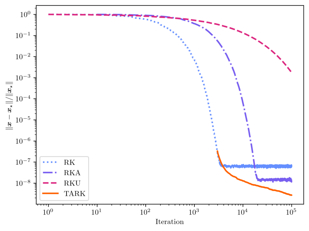
The estimator $\overline{x}_t$ is the tail-averaged randomized Kaczmarz (TARK) estimator. By Theorem 1, we know the TARK estimator has an exponentially small bias:

$\norm{\expect[\overline{x}_t] - x_\star} \le (1 - \kappa_{\rm dem}^{-2})^{2(t_{\rm b}+1)} \norm{x_\star}^2.$

In our paper, we also prove a bound for the mean-square error:

$\expect [\norm{\overline{x}_t - x_\star}^2] \le (1-\kappa_{\rm dem}^{-2})^{t_{\rm b}+1} \norm{x_\star}^2 + \frac{2\kappa_{\rm dem}^4}{t-t_{\rm b}} \frac{\norm{b-Ax_\star}^2}{\norm{A}_{\rm F}^2}.$

We see that the rate of convergence is geometric in the burn-in time $t_{\rm b}$ and occurs at an algebraic, Monte Carlo, rate in the final time $t$ . While the Monte Carlo rate of convergence may be unappealing, it is known that this rate of convergence is optimal for any method that accesses row–entry pairs $(a_i,b_i)$ ; see our paper for a new derivation of this fact.

Tail averaging can be an effective method for squeezing a bit more accuracy out of the RK method for least-squares problems. The figure below shows the error of different RK methods applied to a random least-squares problem, including plain RK, RK with thread averaging (RKA), and RK with underrelaxation (RKU);³ see the paper’s Github for code. For this problem, tail-averaged randomized Kaczmarz achieves the lowest error of all of the methods considered, being 6× smaller than RKA, 22× smaller than RK, and 10⁶× smaller than RKU.

Error versus iteration for different randomized Kaczmarz methods. Tail-averaged randomized Kaczmarz shows the lowest error

What Least-Squares Solution Are We Converging To?

A second implication of Theorem 1 comes from reanalyzing the RK algorithm if we change the sampling probabilities. Recall that the standard RK algorithm draws random row indices $i_t$ using squared row norm sampling:

$\prob \{ i_t = j \} = \frac{\norm{a_j}^2}{\norm{A}_{\rm F}^2} \eqqcolon p^{\rm RK}_j.$

We have notated the RK sampling probability for row $j$ as $p_j^{\rm RK}$ .

Using the standard RK sampling procedure can sometimes be difficult. To implement it directly, we must make a full pass through the matrix to compute the sampling probabilities.⁴ It can be much more convenient to sample rows $i_t$ uniformly at random $\prob \{ i_t = j \} = 1/n$ .

To do the following analysis in generality, consider performing RK using general sampling probabilities $p_j$ :

$\prob \{i_t = j\} = p_j.$

What happens to the bias of the RK iterates then?

Define a diagonal matrix

$D \coloneqq \diag\left( \sqrt{\frac{p_j}{p_j^{\rm RK}}} : j =1,\ldots,n\right).$

One can check that the RK algorithm with non-standard sampling probabilities $\{p_j\}$ is equivalent to the standard RK algorithm run on the diagonally reweighted least-squares problem

$x_{\rm weighted} = \argmin_{x\in\real^d} \norm{Db-(DA)x}.$

In particular, applying TARK with uniform sampling probabilities, the tail-averaged iterates $\overline{x}_t$ will converge to the weighted least-squares problem $x_{\rm weighted}$ rather than the original least-squares solution $x_\star$ .

I find this very interesting. In the standard RK method, the squared row norm sampling distribution is chosen to ensure rapid convergence of the RK iterates to the solution of a consistent system of linear equations. However, for a consistent system, the RK method will always converge to the same solution no matter what row sampling strategy is chosen (as long as every non-zero row has a positive probability of being picked). In the least-squares context, however, the conclusion is very different: the choice of row sampling distribution not only affects the rate of convergence, but also which solution is being converged to!

As the plot below demonstrates, the original least-squares solution and re-weighted least-squares solution can sometimes be quite different from each other. This plot shows the results of fitting a function with many kinks (show as a black dashed curve) using a polynomial function $p(u) = \sum_{j=0}^{10} x_j u^j$ [mfn}Note that, for this experiment we represent the polynomial $p(u) = \sum_{i=0}^{10} x_j u^j$ using its monomial coefficients $x_j$ , which has issues with numerical stability. It’s better to use a representation using Chebyshev polynomials. We use this example only to illustrate the difference between the weighted and original least-squares solution.[/mfn} at $10000$ equispaced points. We compare the unweighted least-squares solution (orange solid curve) to the weighted least-squares solution using uniform RK weights $p_j = 1/n$ (blue dash-dotted curve). These two curves differ meaningfully, with the weighted least-squares solution having higher error at the ends of the interval but more accuracy in the middle. These differences can be explained looking at the weights (diagonal entries of $D$ , grey dotted curve), which are lower at the ends of the interval than in the center.

Weighted and un-weighted least-squares solution to polynomial regression problem. (Tail averaged) randomized Kaczmarz method with uniform sampling converges to the weighted least-squares solution, which is more accurate on the middle of the interval (where the weights are high) than the edges of the interval (where the weights are smaller)

Does this diagonal rescaling issue matter? Sometimes not. In many applications, the weighted and un-weighted least squares solutions will both be fine. Indeed, in the above example, neither the weighted nor un-weighted solutions are the “right” one; the weighted solution is more accurate in the interior of the domain and less accurate at the boundary. However, sometimes getting the true least-squares solution matters, or the amount of reweighting done by uniform sampling is too aggressive for a problem. In these cases, using the classical RK sampling probabilities may be necessary. Fortunately, rejection sampling can often be used to perform squared row norm sampling; see this blog post of mine for details.

Proof of Theorem 1

Let us now prove Theorem 1, the asymptotic unbiasedness of randomized Kaczmarz. We will assume throughout that $A$ is full-rank; the rank-deficient case is similar but requires a bit more care.

Begin by rewriting the update rule in the following way

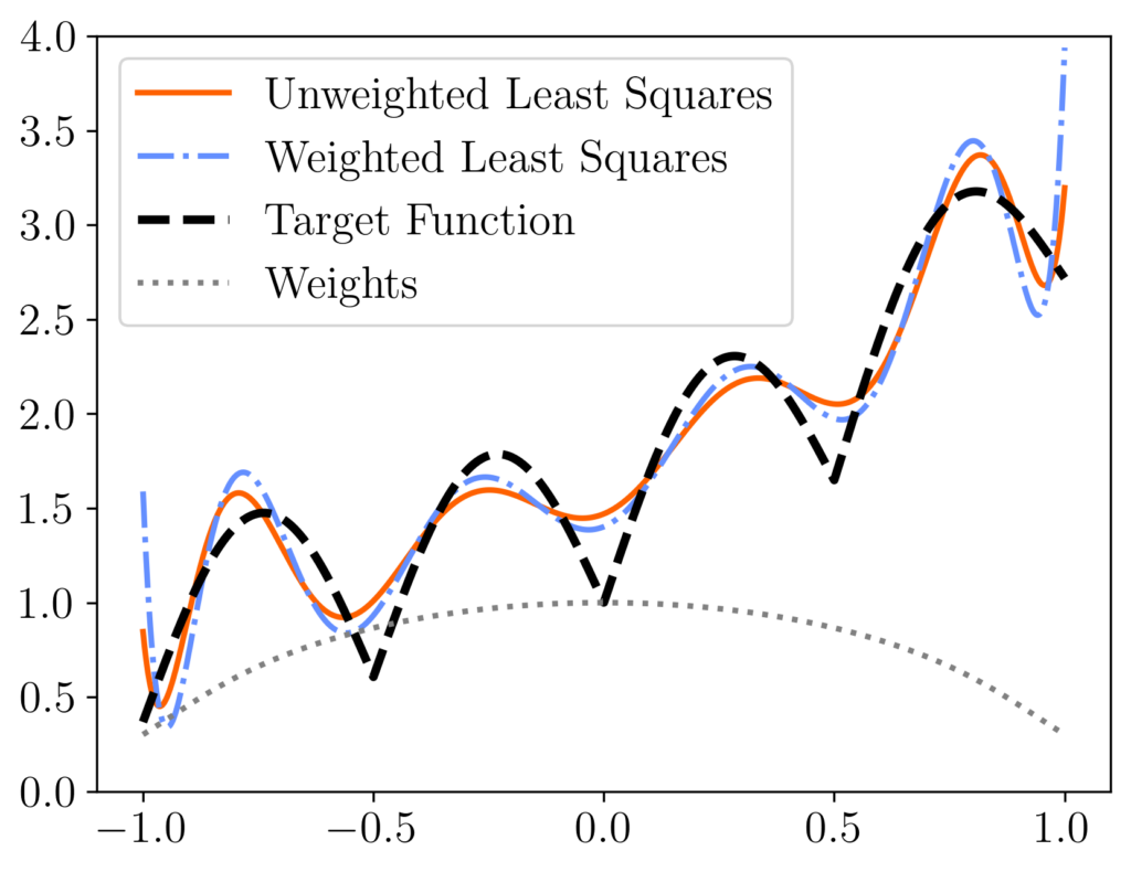
$x_{t+1} = \left( I - \frac{a_{i_t}^{\vphantom{\top}}a_{i_t}^\top}{\norm{a_{i_t}}^2} \right)x_t + \frac{b_{i_t}a_{i_t}}{\norm{a_{i_t}}^2}.$

Now, letting $\expect_{i_t}$ denote the average over the random index $i_t$ , we compute

$\begin{align*}\expect_{i_t}[x_{t+1}] &= \sum_{j=1}^n \left[\left( I - \frac{a_j^{\vphantom{\top}} a_j^\top}{\norm{a_j}^2} \right)x_t + \frac{b_ja_j}{\norm{a_j}^2}\right] \prob\{i_t=j\}\\ &=\sum_{j=1}^n \left[\left( \frac{\norm{a_j}^2}{\norm{A}_{\rm F}^2}I - \frac{a_j^{\vphantom{\top}} a_j^\top}{\norm{A}_{\rm F}^2} \right)x_t + \frac{b_ja_j}{\norm{A}_{\rm F}^2}\right].\end{align*}$

We can evaluate the sums $\sum_{j=1}^n a_j^{\vphantom{\top}}a_j^\top = A^\top A$ and $\sum_{j=1}^n b_j a_j = A^\top b$ directly. Therefore, we obtain

$\expect_{i_t}[x_{t+1}] = \left( I - \frac{A^\top A}{\norm{A}_{\rm F}^2}\right) x_t + \frac{A^\top b}{\norm{A}_{\rm F}^2}.$

Thus, taking the (total) expectation of both sides, we get

$\expect[x_{t+1}] = \left( I - \frac{A^\top A}{\norm{A}_{\rm F}^2}\right) \expect[x_t] + \frac{A^\top b}{\norm{A}_{\rm F}^2}.$

Iterating this equation and using the initial condition $x_0 = 0$ , we obtain

(4) $\expect[x_t] = \left[\sum_{i=0}^{t-1} \left( I - \frac{A^\top A}{\norm{A}_{\rm F}^2}\right)^i \right]\cdot\frac{A^\top b}{\norm{A}_{\rm F}^2}.$

The equation (4) expresses the expected RK iterate $\expect[x_t]$ using a matrix geometric series. Recall that the infinite geometric series with a scalar ratio $|y|<1$ satisfies the formula

$\sum_{i=0}^\infty y^i = (1-y)^{-1}.$

Substituting $x=1-y$ , we get

$\sum_{i=0}^\infty (1-x)^i = x^{-1}$

for any $0 < x < 2$ . With a little effort, one can check that the same formula

$\sum_{i=0}^\infty (I-X)^i = X^{-1}$

for a square matrix $X$ satisfying $0 < \sigma_{\rm min}(X) \le \norm{X} < 2$ . These conditions hold for the matrix $X = A^\top A / \norm{A}_{\rm F}^2$ since $A$ is full-rank, yielding

(5) $\left(\frac{A^\top A}{\norm{A}_{\rm F}^2}\right)^{-1} = \sum_{i=0}^\infty \left( I - \frac{A^\top A}{\norm{A}_{\rm F}^2}\right)^i.$

In anticipation of plugging this result into (4), we can break the infinite sum on the right-hand side into two pieces:

(6) $\left(\frac{A^\top A}{\norm{A}_{\rm F}^2}\right)^{-1} = \sum_{i=0}^{t-1} \left( I - \frac{A^\top A}{\norm{A}_{\rm F}^2}\right)^i + \sum_{i=t}^\infty \left( I - \frac{A^\top A}{\norm{A}_{\rm F}^2}\right)^i.$

We are at the home stretch. Plugging (6) into (4) and using the normal equations $x_\star = (A^\top A)^{-1} A^\top b$ , we obtain

$\expect[x_t] = x_\star - \left[\sum_{i=t}^\infty \left( I - \frac{A^\top A}{\norm{A}_{\rm F}^2}\right)^i \right]\cdot\frac{A^\top b}{\norm{A}_{\rm F}^2}.$

Rearrange to obtain

$\expect[x_t] - x_\star = - \left(I - \frac{A^\top A}{\norm{A}_{\rm F}^2}\right)^t \left[\sum_{i=0}^\infty \left( I - \frac{A^\top A}{\norm{A}_{\rm F}^2}\right)^i \right]\cdot\frac{A^\top b}{\norm{A}_{\rm F}^2}.$

Now apply (5) and the normal equations again to obtain

$\expect[x_t] - x_\star = - \left(I - \frac{A^\top A}{\norm{A}_{\rm F}^2}\right)^t x_\star.$

Take norms and use the submultiplicative property of the spectral norm to obtain

(7) $\norm{\expect[x_t] - x_\star}^2 \le \norm{I - \frac{A^\top A}{\norm{A}_{\rm F}^2}}^{2t} \norm{x}_\star^2.$

To complete the proof we must evaluate the norm of the matrix $I - A^\top A / \norm{A}_{\rm F}^2$ . Let $A = U \Sigma V^\top$ be a (thin) singular value decomposition, where $\Sigma = \diag(\sigma_{\rm max}(A),\ldots,\sigma_{\rm min}(A))$ . Then

$I - \frac{A^\top A}{\norm{A}_{\rm F}^2} = I - V \cdot\frac{\Sigma^2}{\norm{A}_{\rm F}^2} \cdot V^\top = V \left( I - \frac{\Sigma^2}{\norm{A}_{\rm F}^2}\right)V^\top.$

We recognize this as a matrix whose eigenvectors are $V$ and whose eigenvalues are the diagonal entries of the matrix

$I - \Sigma^2/\norm{A}_{\rm F}^2 = \diag(1 - \sigma^2_{\rm max}(A)/\norm{A}_{\rm F}^2,\ldots,1-\sigma_{\rm min}^2(A)/\norm{A}_{\rm F}^2).$

All eigenvalues are nonnegative and the largest eigenvalue is $1 - \sigma_{\rm min}^2(A)/\norm{A}_{\rm F}^2 = 1 - \kappa_{\rm dem}^{-2}$ . We have invoked the definition of the Demmel condition number (2). Therefore, plugging into (7), we obtain

$\norm{\expect[x_t] - x_\star}^2 \le \left(1-\kappa_{\rm dem}^{-2}\right)^{2t} \norm{x}_\star^2,$

as promised.

Note to Self: Sketch-and-Solve with a Gaussian Embedding

November 19, 2024 by Ethan N. Epperly Leave a comment

In the comments to my post Does Sketching Work?, I was asked a very interesting question, which I will paraphrase as follows:

Is the sketch-and-solve least-squares solution $\hat{x} = \operatorname*{argmin}_{\hat{x}} \norm{(SA)\hat{x} - Sb}$ an unbiased estimate of the true least squares solution of $x = \operatorname*{argmin}_x \norm{Ax - b}$ ?

In this post, I will answer this question for the special case in which $S$ is a Gaussian sketch, and I will also compute the expected least-squares residual $\expect \norm{A\hat{x}-b}^2$ . Throughout this post, I will assume knowledge of sketching; see my previous two posts for a refresher if needed. For this post, $A$ will have dimensions $n\times d$ and $S$ will have dimensions $\ell\times n$ , and these parameters are related $n\ge \ell \ge d$ .

I thought I knew the answer to this question—that sketch-and-solve suffers from inversion bias. Indeed, the fact I remembered is that

(1) $\expect\Big[\big((SA)^\top (SA)\big)^{-1}\Big] \ne \big(A^\top A\big)^{-1}$

for the sketching matrices $S$ in common use. The issue of the inversion bias (1) is discussed in this paper.

However, the inversion bias (1) does not imply that sketch-and-solve is biased. In fact, for a Gaussian sketch¹

(2) $S \in \real^{\ell\times n} \quad \text{with } S_{ij} \sim \text{Normal}(0,1) \text{ iid},$

sketch-and-solve is unbiased.

Theorem (Gaussian sketch-and-solve is unbiased). Let $S$ be a Gaussian sketch (2) and let $A \in \real^{n\times d}$ be a full column-rank matrix. Then
(3) $\expect[(SA)^\dagger(Sb)] = A^\dagger b.$
That is, the sketch-and-solve solution $(SA)^\dagger(Sb)$ is an unbiased estimate for the least-squares solution $A^\dagger b$ .

Here, ${}^\dagger$ is the Moore–Penrose pseudoinverse, which effectuates the least-squares solution:

$A^\dagger b = \operatorname*{argmin}_{x\in\real^d} \norm{Ax - b}.$

In particular, by the normal equations, we have the relation

(4) $A^\dagger = (A^\top A)^{-1} A^\top,$

valid for any matrix $A$ with full column-rank.

Let us prove this theorem. The Gaussian sketch (1) is orthogonally invariant: that is, $V^\top SU$ has the same distribution as $S$ for any orthogonal matrices $U$ and $V$ . Thus, we are free to reparametrize. Let

$A = U\twobyone{\Sigma}{0}V^\top$

be a (full) singular value decomposition of $A$ . Make the changes of variables

$A \mapsto U^\top A V, \quad S \mapsto V^\top SU, \quad b \mapsto U^\top b.$

After this change of variables, $S$ still has the same distribution (2) and

$A = \twobyone{\Sigma}{0}.$

Partition the reparametrized $b$ and $S$ conformally with $A$ :

$b = \twobyone{b_1}{b_2}, \quad S = \onebytwo{S_1}{S_2}.$

Under this change of variables, the least-squares solution is

(5) $A^\dagger b = \Sigma^{-1}b_1.$

Now, we are ready to prove the claim (3). Observe that $SA = S_1\Sigma$ . Begin by using the normal equations (4) to write out the sketch-and-solve solution

$(SA)^\dagger (Sb) = [(SA)^\top (SA)]^{-1}(SA)^\top (Sb).$

Observe that $SA = S_1\Sigma$ . Thus,

$(SA)^\dagger (Sb) = [\Sigma S_1^\top S_1\Sigma]^{-1}\Sigma S_1^\top \onebytwo{S_1}{S_2}\twobyone{b_1}{b_2}.$

Simplify to obtain

$(SA)^\dagger (Sb) = \Sigma^{-1}(S_1^\top S_1)^{-1} S_1^\top (S_1b_1 + S_2 b_2).$

Using the normal equations (4) and the solution formula (5), we obtain

(6) $(SA)^\dagger (Sb) = \Sigma^{-1}b_1 + \Sigma^{-1} S_1^\dagger S_2b_2 = A^\dagger b + \Sigma^{-1} S_1^\dagger S_2b_2.$

By the definition (2) of $S$ , $S_1$ and $S_2$ are independent and $\expect[S_2] = 0$ . Thus, taking expectations, we obtain

$\expect[(SA)^\dagger (Sb)] = A^\dagger b + \Sigma^{-1} \expect[S_1^\dagger] \expect[S_2]b_2 = A^\dagger b.$

The desired claim (3) is proven.

Note that the solution formula (6) holds for any sketching matrix $S$ . We only use Gaussianity at the last step, where we invoke three properties (1) $S$ is mean zero; (2) $S$ is orthogonally invariant; and (3) conditional on the first $d$ columns of $S$ , the last $n-d$ columns of $S$ are mean-zero.

The Least-Squares Residual for Gaussian Sketch-and-Solve

The solution formula (6) can be used to understand other properties of the Gaussian sketch-and-solve solution. In this section, we use (6) to understand the expected squared residual norm

$\expect \norm{A\hat{x} - b}^2,$

where $\hat{x} = (SA)^\dagger (Sb)$ is the sketch-and-solve solution. We write the expected residual norm as

$\expect\norm{A\hat{x} - b}^2 = \expect\norm{\twobyone{b_1 + S_1^\dagger S_2b_2}{0} - \twobyone{b_1}{b_2}}^2 = \norm{b_2}^2 + \expect\norm{S_1^\dagger S_2b_2}^2.$

Now, use the Gaussian–inverse Gaussian matrix product formula to compute the expectation, obtaining

$\expect\norm{A\hat{x} - b}^2 = \left(1+\frac{d}{\ell-d-1}\right)\norm{b_2}^2.$

Finally, we recognize $\norm{b_2}$ is the optimal least-squares residual $\min_x \norm{Ax - b}$ . Thus, we have shown

$\expect\norm{A\hat{x} - b}^2 = \left(1+\frac{d}{\ell-d-1}\right)\min_{x\in\real^d} \norm{Ax-b}^2.$

Note that this is an exact formula for the expected squared residual for the sketch-and-solve solution! Thus, the sketch-and-solve solution has an expected squared residual that factor $1 + d/(\ell-d-1)$ larger than the optimal value. In particular,

$\expect\norm{A\hat{x} - b}^2 = \left(1+\varepsilon\right)\min_{x\in\real^d} \norm{Ax-b}^2 \quad \text{when } \ell = \frac{d}{\varepsilon} + d + 1.$

Remark (Existing literature): When I originally wrote this post, I had not seen these results anywhere in the literature. Thanks to Michał Dereziński, who provided me with the following references: the following lecture notes of Mert Pilanci, equation 1 in this recent paper of Michał’s, and this recent survey by Michał and Michael Mahoney. I find it striking that these basic and beautiful results appear to only have been explicitly recorded very recently. Very big thanks also to Rob Webber for providing help in preparing this post.

Update (11/21/24): After this post was initially released, Mert Pilanci provided me with an earlier reference (2020); see also this paper for extensions. He also mentions an even earlier paper (2017) that does similar calculations in a statistical setting, but does not obtain exactly these formulas. See also this paper for exact and asymptomatically exact formulas for sketch-and-solve in the statistical setting.

Note to Self: Hanson–Wright and Trace Estimation with Random Vectors on the Sphere

November 4, 2024 by Ethan N. Epperly Leave a comment

Tyler Chen has just released an excellent monograph on the Lanczos method, one of the most powerful algorithms for extracting information from a symmetric matrix $A$ . I would definitely recommend checking it out.

One of the subjects touched on by this book is stochastic trace estimation, a topic I’ve written about several times before on this blog. In his book, Tyler uses stochastic trace estimates based on random vectors on the sphere (a great choice), and he provides a simple, but often pessimistic, mathematical analysis of this approach. To complement Tyler’s amazing book, I felt it was a good opportunity to share a sharper analysis that I came up with using a more sophisticated argument. I would not be surprised if this argument appears elsewhere in the literature, but I am not aware of a source.

Let $x,x_1,\ldots,x_m$ be random vectors in $\real^n$ drawn uniformly at random from the sphere of radius $\sqrt{n}$ ,¹ let $A$ be a real symmetric matrix, and define the quadratic form

$q \coloneqq x^\top Ax$

and the Girard–Hutchinson trace estimator

$\hat{\tr}\coloneqq \frac{1}{m}\sum_{i=1}^m x_i^\top Ax_i.$

Both $q$ and $\hat{\tr}$ are unbiased estimates for the trace of $A$ , $\expect[q] = \expect[\hat{\tr}] = \tr A$ . The goal of this post will be to bound the probability of these quantities being much smaller or larger than the trace of $A$ .

Hanson–Wright on the Sphere

Observe that $\hat{\tr}$ is an average of $m$ independent copies of the random variable $q$ . Therefore, we will begin our analysis with the quadratic form $q$ and discuss the Girard–Hutchinson estimate $\hat{\tr}$ at the end of the post.

Centering

Begin by introducing the centered matrix

$\overline{A} = A - \frac{\tr A}{n}I.$

The transformation $A\mapsto\overline{A}$ has the effect of shifting $A$ ’s eigenvalues to have mean zero. Consequently, since the trace is the sum of the eigenvalues, $\overline{A}$ has trace zero.

Now, rewrite $q$ in terms of the centered matrix $\overline{A}$ :

$q = x^\top A x = x^\top \overline{A} x + \frac{\tr A}{n} \cdot x^\top I x = x^\top \overline{A} x + \tr A.$

In the final equality, we use the fact that $x$ is on the sphere of radius $\sqrt{n}$ so that $x^\top I x = \norm{x}^2 = n$ . Rearranging, we see that the error $\overline{q}\coloneqq q-\tr A$ satisfies

$\overline{q} = q-\tr A = x^\top \overline{A}x.$

We have shown that the error $\overline{q}$ depends only on the centered matrix $\overline{A}$ rather than the original matrix $A$ . This observation is at the root of the reason that quadratic forms with vectors on the sphere have smaller tail probabilities than other distributions like the Gaussian distribution. Indeed, $\overline{A}$ is smaller than $A$ when measured using the Frobenius norm $\norm{\overline A}_{\rm F} \le \norm{A}_{\rm F}$ , and the spectral norm is never much larger $\norm{\overline{A}} \le 2\norm{A}$ . These observations will be important later.

Laplace Transform Method and Comparison to Standard Gaussian Vectors

To derive exponential concentration inequalities, we make use of the Laplace transform method. For a random variable $z$ , define the cumulant generating function (cgf)

$\xi_z(\theta) = \log (\expect [\exp(\theta z)]).$

Bounds on the cgf immediately yield bounds on the random variable taking large values, so it will behoove us to estimate this quantity for $\overline{q}$ .

To estimate the cgf of $\overline{q}$ , we will make use of a comparison between Gaussian vectors and random vectors on the sphere. Recall that a standard Gaussian vector $g$ is a vector with independent standard Gaussian entries. Standard Gaussian random vectors are spherically symmetric, meaning they can be written in the form $g = a\cdot x$ , where $x$ is a uniform random vector on the sphere and $a$ is a scaling factor.² The scaling factor $a$ is independent of $x$ and, in this case, satisfies $\expect[a^2] = 1$ .³

Using this relationship, the error $\overline{q}$ can be connected to the standard Gaussian random vector $g$ as follows

$g^\top \overline{A} g = a^2 \cdot x^\top \overline{A} x = a^2 \cdot \overline{q}.$

Intuitively, we might expect that multiplying the random error $\overline{q}$ by a scaling factor of mean one should only have the effect of increasing the variability of $\overline{q}$ and thus increasing its probability of taking large values. Based on this intuition, we might conjecture that the cgfs are related

$\xi_{\overline{q}}(\theta) \le \xi_{g^\top A g}(\theta) \quad \text{for all } \theta \in \real.$

Indeed, this conjecture is true.

Proposition (Scaling hurts). Let $z$ be a random variable and let $b$ be a random variable with expectation $1$ , independent of $z$ . Then
$\xi_{z}(\theta) \le \xi_{bz}(\theta) \quad \text{for all } \theta \in \real.$

To prove this result, let $\expect_b$ and $\expect_z$ denote expectations take over the randomness in $b$ and $z$ separately. The total expectation is $\expect[\cdot] = \expect_z[\expect_b[\cdot ]]$ . Begin with the right-hand side and invoke Jensen’s inequality over $b$ :

$\xi_{bz}(\theta) = \xi_z(\theta) = \log (\expect_z [\expect_b [\exp(\theta bz)]]) \ge \log (\expect_z [\exp(\theta \expect_b[b]z)]) = \xi_z(\theta).$

In the last line, we use the hypothesis $\expect[b] = 1$ and the definition of the cgf.

Having established this proposition, we conclude that $\xi_{\overline{q}}(\theta) \le \xi_{g^\top \overline{A} g}(\theta)$ for all $\theta$ .

Completing the Analysis

Finally, invoking a standard bound for the cgf of $g^\top \overline{A}g$ for a trace-zero matrix $\overline{A}$ , we obtain

$\xi_{\overline{q}}(\theta) \le \xi_{g^\top \overline{A} g}(\theta) \le \frac{\theta^2 \norm{\overline{A}}_{\rm F}^2}{1 - 2\theta \norm{\overline{A}}}.$

A cgf bound of this form immediately yields the following tail bound (see Boucheron, Lugosi, and Massart’s Concentration Inequalities page 29 and Exercise 2.8):

$\prob \{ x^\top A x - \tr(A) \ge t \} \le \exp \left( - \frac{t^2/2}{2 \norm{\overline{A}}_{\rm F}^2 + 2 \overline{\norm{\overline{A}}t}} \right).$

One can also control the lower tail event $x^\top A x - \tr(A) \le -t$ by instantiating this result with $-A$ . Union bounding over the upper and lower tails gives the symmetric bound

$\prob \{ |x^\top A x - \tr(A)| \ge t \} \le 2\exp \left( - \frac{t^2/2}{2 \norm{\overline{A}}_{\rm F}^2 + 2 \overline{\norm{\overline{A}}t}} \right).$

Is This Bound Good?

Tail bounds for quadratic forms such as $x^\top A x$ or $g^\top A g$ are known as Hanson–Wright inequalities. For vectors on the sphere, our bound shows the tail probabilities decay like $\exp(-O(t^2/\norm{\overline{A}_{\rm F}}^2))$ for small $t > 0$ and $\exp(-O(t/\norm{\overline{A}}))$ for large $t>0$ . This pattern of results “subgaussian scaling for small $t$ , subexponential scaling for large $t$ ” is typical for Hanson–Wright inequalities.

The Hanson–Wright inequalities for vectors on the sphere exhibit faster decay rate than for standard Gaussian vectors. Indeed, a standard Gaussian random vector $g$ obeys a Hanson–Wright inequality of the form

$\prob \{ g^\top A g - \tr A \ge t \} \le \exp \left( -\frac{t^2/2}{C\norm{A}_{\rm F}^2 + c t \norm{A}}\right)$

for positive constants $C,c > 0$ . For vectors on the sphere, $\norm{A}_{\rm F}^2$ and $\norm{A}$ have been replaced by $\norm{\overline{A}}_{\rm F}^2$ and $\norm{\overline{A}}$ which are always smaller (and sometimes much smaller). The smaller tail probabilities for $x^\top A x$ versus $g^\top A g$ is a real phenomenon, not an artifact of the mathematical analysis.

As another way to evaluate the quality of these bounds, recall that a Gaussian random variable with mean zero and variance $v$ has tail probabilities roughly of size $\exp(-t^2/2v)$ . For small $t$ , our Hanson–Wright inequality for vectors on the sphere has the same form with $v = 2\norm{\overline{A}}_{\rm F}^2$ . The true variance of $q = x^\top A x$ is

$\Var(q) = \frac{n}{n+2} \cdot 2\norm{\overline{A}}_{\rm F}^2,$

which is close to $v = 2\norm{\overline{A}}_{\rm F}^2$ for large $n$ . (See this post of mine for a derivation of the variance formula.) Thus, even up to the constants, the Hanson–Wright inequality we’ve derived for random vectors on the sphere is nearly as good as one could possibly hope (at least for small $t$ ).

Girard–Hutchinson Estimator on the Sphere

Using our results for one quadratic form, tail bounds for the Girard–Hutchinson estimator $\overline{\tr} = m^{-1} \sum_{i=1}^m x_i^\top A x_i$ easily follow. Indeed, the cgf is additive for independent random variables and satisfies the identity $\xi_{cz}(\theta) = \xi_z(c\theta)$ for constant $c, so

$\xi_{\overline{\tr}}(\theta) = \sum_{i=1}^m \xi_{x_i^\top Ax_i}(\theta/m) \le m \cdot \frac{(\theta/m)^2 \norm{\overline{A}}_{\rm F}^2}{1 - 2(\theta/m)\norm{\overline{A}}}.$

This cgf bound leads to tail bounds

$\begin{align*}\prob \{ \overline{\tr} - \tr(A) \ge t \} &\le \exp \left( - \frac{mt^2/2}{2\norm{\overline{A}}_{\rm F}^2 + 2m \overline{\norm{\overline{A}}t}} \right), \\\prob \{ |\overline{\tr} - \tr(A)| \ge t \} &\le 2\exp \left( - \frac{mt^2/2}{2\norm{\overline{A}}_{\rm F}^2 + 2m \overline{\norm{\overline{A}}t}} \right).\end{align*}$

Rejection Sampling

October 8, 2024 by Ethan N. Epperly 3 Comments

I am delighted to share that my paper Embrace rejection: Kernel matrix approximation with randomly pivoted Cholesky has been released on arXiv, joint with Joel Tropp and Rob Webber.

On the occasion of this release, I want to talk about rejection sampling, one of the most powerful ideas in probabilistic computing. My goal is to provide an accessible and general introduction to this technique, with a more “applied math” rather than statistical perspective. I will conclude with some discussion of how we use it in our paper.

Motivating Application: Randomized Kaczmarz

Consider the task of solving a linear system of equations $Ax = b$ , where $A \in \real^{n\times d}$ is a matrix and $b \in \real^n$ is a vector. For simplicity, we assume that this system is consistent (i.e., there exists a solution $x_\star$ such that $Ax_\star = b$ ). The randomized Kaczmarz algorithm is a mathematically elegant algorithm for solving this problem, due to Strohmer and Vershynin. Beginning with initial solution $x \gets 0$ , randomized Kaczmarz repeatedly performs the following steps:

Sample. Generate a random row index $I$ according to the probability distribution $\prob \{I = i\} = \norm{a_i}^2 / \norm{A}_{\rm F}^2$ . Here, and going forward, $a_i^\top$ denotes the $i$ th row of $A$ and $\norm{\cdot}_{\rm F}$ is the Frobenius norm.
Update. Set $x \gets x + (b_I - a_I^\top x)\cdot a_I / \norm{a_I}^2$ .

Convergence theory of the randomized Kaczmarz iteration is very well-studied; see, e.g., section 4.1 of this survey for an introduction.

For this post, we will consider a more basic question: How can we perform the sampling step 1? If $n$ and $d$ are not very large, this is an easy problem: Simply sweep through all the rows $a_i$ and compute their norms $\norm{a_i}^2$ . Then, sampling can be done using any algorithm for sampling from a weighted list of items. But what if $n$ is very large? Suppose, even, that it is computationally expensive to read through the matrix, even once, to compute the row norms. What can we do now?

Here is one solution is using rejection sampling, due to Needell, Ward, and Srebro. Suppose that we know a bound on the row norms of $A$ :

(1) $\norm{a_i}^2 \le B \quad \text{for each } i = 1,\ldots,n.$

For instance, if the entries of $A$ take values in the range $[-1,1]$ , then (1) holds with $B = d$ . To sample a row $i$ with probability $\norm{a_i}^2/\norm{A}_{\rm F}^2$ , we perform the following the rejection sampling procedure:

Propose. Draw a random row index $1\le J\le n$ uniformly at random (i.e., $J$ is equally likely to be any row index between $1$ and $n$ .)
Accept/reject. Make a random choice: With probability $p_J = \norm{a_J}^2/B$ , accept and set $I\gets J$ . With the remaining probability $1-p_J$ , reject and return to step 1.

Why does this procedure work? As an intuitive explanation, notice that each row $i$ is equally likely to be proposed and has probability proportional to $\norm{a_i}^2$ of being accepted. Therefore, under this procedure, each row $i$ has probability proportional to $\norm{a_i}^2$ of being selected, just as desired for randomized Kaczmarz. If this intuitive justification is unsatisfying, we’ll have a formal derivation of correctness below (in a more general context).

I find rejection sampling to be super neat. In this case, it allows us to use simple ingredients (uniform row sampling and an upper bound on the row norms) to accomplish a more complicated task (sampling according to the squared row norms). We can sample from an interesting probability distribution (the squared row norm distribution) by thinning out samples from a simple distribution. This is a powerful idea that has many applications. (And, I believe, many more applications are waiting to be discovered.)

Rejection Sampling in General

Let’s now discuss rejection sampling in a bit more generality. Say I have a list of $n$ things each of which has a weight $w_i\ge 0$ . Our goal is to choose a random index $I$ with probability proportional to $w_i$ , i.e., $\prob \{ I = i\} = w_i / \sum_{j=1}^n w_j$ . We will call $w$ the target distribution. (Note that we do not require the weights $w_i$ to be normalized to satisfy $\sum_{i=1}^n w_i =1$ .)

Suppose that sampling from the target distribution is challenging, but we can sample from a proposal distribution $\rho$ , i.e., we can efficiently generate random $J$ such that $\prob \{J = i\} = \rho_i / \sum_{j=1}^n \rho_j$ . Further, suppose that the proposal distribution dominates the target distribution in the sense that

$w_i \le \rho_i \quad \text{for each } i=1,\ldots,n.$

Under this general setting, we can sample $I$ from the target distribution using rejection sampling, similar to above:

Propose. Draw a random row index $J$ from the proposal distribution.
Accept/reject. Make a random choice: With probability $p_J = w_J/\rho_J$ , accept and set $I\gets J$ . With the remaining probability $1-p_J$ , reject and return to step 1.

We recognize the squared row-norm sampling above as an example of this general strategy with $w_i = \norm{a_i}^2$ and $\rho_i = B$ for all $i$ .

Let us now convince ourselves more carefully that rejection sampling works. On any given execution of the rejection sampling loop, the probability of proposing index $i$ is $\rho_i / \sum_{j=1}^n \rho_j$ , after which the probability of accepting $i$ is $w_i / \rho_i$ . Therefore, the probability of outputting $i$ at any given loop is

$\prob \{\text{$i$ accepted this loop}\} = \frac{\rho_i}{\sum_{j=1}^n \rho_j} \cdot \frac{w_i}{\rho_i} = \frac{w_i}{\sum_{j=1}^n \rho_j}.$

The probability that any index $i$ on that loop is accepted is thus

$\prob \{\text{any accepted this loop}\} = \sum_{i=1}^n \prob \{\text{$i$ accepted this loop}\} = \frac{\sum_{i=1}^n w_i}{\sum_{i=1}^n \rho_i}.$

The rejection sampling loop accepts with fixed positive probability each execution, so it eventually accepts with 100% probability. Thus, the probability of accepting $i$ conditional on some index being accepted is

$\prob \{\text{$i$ accepted this loop} \mid \text{any accepted this loop}\} = \frac{\prob \{\text{$i$ accepted this loop}\}}{\prob \{\text{any accepted this loop}\}} = \frac{w_i}{\sum_{j=1}^n w_j}.$

Therefore, rejection sampling outputs a sample $I$ from the target distribution $w$ as promised.

As this analysis shows, the probability of accepting on any given execution of the rejection sampling loop is $\sum_{i=1}^n w_i / \sum_{i=1}^n \rho_i$ , the ratio of the total mass of the target $w_i$ to the total mass of the proposal $\rho_i$ . Thus, rejection sampling will have a high acceptance rate if $w_i \approx \rho_i$ and a low acceptance rate if $w_i \ll \rho_i$ . The conclusion for practice is that rejection sampling is only computationally efficient if one has access to a good proposal distribution $\rho_i$ , that is both easy to sample from and close to the target $w_i\approx \rho_i$ .

Here, we have presented rejection sampling as a strategy for sampling from a discrete set of items $i=1,\ldots,n$ , but this not all that rejection sampling can do. Indeed, one can also use rejection sampling for sampling a real-valued parameters $x \in \real$ or a multivariate parameter $x \in \real^n$ from a given (unnormalized) probability density function (or, if one likes, an unnormalized probability measure).

Before moving on, let us make one final observation. A very convenient thing about rejection sampling is that we only need the unnormalized probability weights $w_i$ and $\rho_i$ to implement the procedure, even though the total weights $\sum_{j=1}^n w_i$ and $\sum_{j=1}^n \rho_i$ are necessary to define the sampling probabilities $\prob \{I = i\} = w_i / \sum_{j=1}^n w_j$ and $\prob \{J = i\} = \rho_i / \sum_{j=1}^n \rho_j$ . This fact is necessary for many applications of rejection sampling. For instance, in the randomized Kaczmarz use, rejection sampling would be much less useful if we needed the total weight $\sum_{i=1}^n \norm{a_i}^2 = \norm{A}_{\rm F}^2$ , as computing $\norm{A}_{\rm F}^2$ requires a full pass over the data to compute.

Application: Randomly pivoted Cholesky

Another application of rejection sampling appears is to accelerate the randomly pivoted Cholesky algorithm, the subject of my recent paper. Here, I’ll provide an overview of the main idea with a focus on the role of rejection sampling in the procedure. See the paper for more details. Warning: Even as simplified here, this section presents a significantly more involved application of rejection sampling than we saw previously with randomized Kaczmarz!

Randomly pivoted Cholesky (RPCholesky) is a simple, but powerful algorithm for computing a low-rank approximation to a symmetric positive semidefinite matrix $A$ , and it can be used to accelerate kernel machine learning algorithms.

Conceptually, RPCholesky works as follows. Let $A^{(0)} \coloneqq A$ denote the initial matrix and $\hat{A}^{(0)} \coloneqq 0$ denote a trivial initial approximation. For $j=0,1,2,\ldots,k-1$ , RPCholesky performs the following steps:

Random sampling. Draw a random index $I_{j+1}$ with probability $\prob \{ I_{j+1} = i\} = A^{(j)}_{ii} / \sum_{i=1}^n A^{(j)}_{ii}$ .
Update approximation. Update $\hat{A}^{(j+1)} \gets \hat{A}^{(j)} + a_i^{(j)}(a_i^{(j)})^\top / A_{ii}^{(j)}$ . Here, $a_i^{(j)}$ denotes the $i$ th column of $A^{(j)}$ .
Update matrix. Update $A^{(j+1)} \gets A^{(j)} + a_i^{(j)}(a_i^{(j)})^\top / A_{ii}^{(j)}$ .

The result of this procedure is a rank- $k$ approximation $\hat{A}^{(k)}$ . With an optimized implementation, RPCholesky requires only $O(k^2N)$ operations and evaluates just $(k+1)N$ entries of the input matrix $A$ .

The standard RPCholesky algorithm is already fast, but there is room for improvement. The standard RPCholesky method processes the matrix $A$ one column $a_i$ at a time, but modern computers are faster at processing blocks of columns. Using the power of rejection sampling, we can develop faster versions of RPCholesky that take advantage of blocked computations. These blocked implementations are important: While we could handle a million-by-million matrix using the standard RPCholesky method, blocked implementations can be up to 40 $\times$ faster. In this post, I’ll describe the simplest way of using rejection sampling to implement RPCholesky.

To set the stage, let’s first establish some notation and make a few observations. Let $S_j = \{I_1,\ldots,I_j\}$ denote the first $j$ selected random indices. With a little matrix algebra, one can show that the approximation $\hat{A}^{(j)}$ produced by $j$ steps of RPCholesky obeys the formula¹

(1) $\hat{A}^{(j)} = A(:,S_j) A(S_j,S_j)^{-1}A(S_j,:).$

Here, we are using MATLAB notation for indexing the matrix $A$ . The residual matrix $A^{(j)}$ is given by

$A^{(j)} = A - \hat{A}^{(j)} = A - A(:,S_j) A(S_j,S_j)^{-1}A(S_j,:).$

Importantly for us, observe that we can evaluate the $i$ th diagonal entry of $A^{(j)}$ using the formula

(2) $A^{(j)}_{ii} = A_{ii} - A(i,S_j) A(S_j,S_j)^{-1} A(S_j,i).$

Compared to operating on the full input matrix $A$ , evaluating an entry $A^{(j)}_{ii}$ is cheap, just requiring some arithmetic involving matrices and vectors of size $j$ .

Here, we see a situation similar to randomized Kaczmarz. At each step of RPCholesky, we must sample a random index $I_{j+1}$ from a target distribution $w_i = A_{ii}^{(j)}$ , but it is expensive to evaluate all of the $w_i$ ‘s. This is a natural setting for rejection sampling. As proposal distribution, we may use the initial diagonal of $A$ , $\rho_i = A_{ii}$ . (One may verify that, as required, $w_i = A_{ii}^{(j)} \le A_{ii} = \rho_i$ for all $i$ .) This leads to a rejection sampling implementation for RPCholesky:

Sample indices. For $j=0,1,\ldots,k-1$ , sample random indices $I_{j+1}$ from the target distribution $w_i = A^{(j)}_{ii}$ using rejection sampling with proposal distribution $\rho_i = A_{ii}$ . Entries $A_{ii}^{(j)}$ are evaluated on an as-needed basis using (2).
Build the approximation. Form the approximation $\hat{A}^{(k)}$ all at once using (1).

By using rejection sampling, we have gone from an algorithm which handles the matrix one column at a time to a new algorithm which processes columns of the matrix $A$ all at once through the formula (1). In the right situations, this new algorithm can be significantly faster than the original RPCholesky method.²

We have now seen two extreme cases: the standard RPCholesky algorithm that processes the columns of $A$ one at a time and a rejection sampling implementation that operates on the columns of $A$ all at once. In practice, the fastest algorithm sits between these extremes, using rejection sampling to sample column indices in moderate-size blocks (say, between 100 and 1000 columns at a time). This “goldilocks” algorithm is the accelerated RPCholesky method that we introduce in our paper. Check it out for details!

Conclusion: Rejection Sampling, an Algorithm Design Tool

We’ve now seen two applications, randomized Kaczmarz and randomly pivoted Cholesky, where rejection sampling can be used to speed up an algorithm. In both cases, we wanted to sample from a distribution over $n$ row or column indices, but it was expensive to perform a census to compute the probability weight of each item individually. Rejection sampling offers a different approach, where we generate samples from a cheap-to-sample proposal distribution and only evaluate the probability weights of the proposed items. In the right situations, this rejection sampling approach can lead to significant computational speedups.

Rejection sampling has been used by statistics-oriented folks for decades, but the power of this technique seems less well-known to researchers in applied math, scientific computation, and related areas. I think there are a lot more exciting ways that we can use rejection sampling to design better, faster randomized algorithms.

Neat Randomized Algorithms: RandDiag for Rapidly Diagonalizing Normal Matrices

July 2, 2024 by Ethan N. Epperly Leave a comment

Consider two complex-valued square matrices $A\in\complex^{n\times n}$ and $B\in\complex^{n\times n}$ . The first matrix $A$ is Hermitian, being equal $A = A^*$ to its conjugate transpose $A^*$ . The other matrix $B$ is non-Hermitian, $B \ne B^*$ . Let’s see how long it takes to compute their eigenvalue decompositions in MATLAB:

>> A = randn(1e3) + 1i*randn(1e3); A = (A+A')/2;
>> tic; [V_A,D_A] = eig(A); toc % Hermitian matrix
Elapsed time is 0.415145 seconds.
>> B = randn(1e3) + 1i*randn(1e3);
>> tic; [V_B,D_B] = eig(B); toc % non-Hermitian matrix
Elapsed time is 1.668246 seconds.

We see that it takes $4\times$ longer to compute the eigenvalues of the non-Hermitian matrix $B$ as compared to the Hermitian matrix $A$ . Moreover, the matrix $V_A$ of eigenvectors for a Hermitian matrix $A = V_AD_AV_A^{-1}$ is a unitary matrix, $V_A^*V_A = V_AV_A^* = I$ .

There are another class of matrices with nice eigenvalue decompositions, normal matrices. A square, complex-valued matrix $C$ is normal if $C^*C = CC^*$ . The matrix $V_C$ of eigenvectors for a normal matrix $C = V_C D_C V_C^{-1}$ is also unitary, $V_C^*V_C = V_CV_C^* = I$ . An important class of normal matrices are unitary matrices themselves. A unitary matrix $U$ is always normal since it satisfies $U^*U = UU^* = I$ .

Let’s see how long it takes MATLAB to compute the eigenvalue decomposition of a unitary (and thus normal) matrix:

>> U = V_A;                     % unitary, and thus normal, matrix
>> tic; [V_U,D_U] = eig(U); toc % normal matrix
Elapsed time is 2.201017 seconds.

Even longer than it took to compute an eigenvalue decomposition of the non-normal matrix $B$ ! Can we make the normal eigenvalue decomposition closer to the speed of the Hermitian eigenvalue decomposition?

Here is the start of an idea. Every square matrix $C$ has a Cartesian decomposition:

$C = H + iS, \quad H = \frac{C+C^*}{2}, \quad S = \frac{C-C^*}{2i}.$

We have written $C$ as a combination of its Hermitian part $H$ and $i$ times its skew-Hermitian part $S$ . Both $H$ and $S$ are Hermitian matrices. The Cartesian decomposition of a square matrix is analogous to the decomposition of a complex number into its real and imaginary parts.

For a normal matrix $C$ , the Hermitian and skew-Hermitian parts commute, $HS = SH$ . We know from matrix theory that commuting Hermitian matrices are simultaneously diagonalizable, i.e., there exists $Q$ such that $H = QD_HQ^*$ and $S = QD_SQ^*$ for diagonal matrices $D_H$ and $D_S$ . Thus, given access to such $Q$ , $C$ has eigenvalue decomposition

$C = Q(D_H+iD_S)Q^*.$

Here’s a first attempt to turn this insight into an algorithm. First, compute the Hermitian part $H$ of $C$ , diagonalize $H = QD_HQ^*$ , and then see if $Q$ diagonalizes $C$ . Let’s test this out on a $2\times 2$ example:

>> C = orth(randn(2) + 1i*randn(2)); % unitary matrix
>> H = (C+C')/2;                     % Hermitian part
>> [Q,~] = eig(H);
>> Q'*C*Q                            % check to see if diagonal
ans =
  -0.9933 + 0.1152i  -0.0000 + 0.0000i
   0.0000 + 0.0000i  -0.3175 - 0.9483i

Yay! We’ve succeeded at diagonalizing the matrix $C$ using only a Hermitian eigenvalue decomposition. But we should be careful about declaring victory too early. Here’s a bad example:

>> C = [1 1i;1i 1]; % normal matrix
>> H = (C+C')/2;
>> [Q,~] = eig(H);
>> Q'*C*Q           % oh no! not diagonal
ans =
   1.0000 + 0.0000i   0.0000 + 1.0000i
   0.0000 + 1.0000i   1.0000 + 0.0000i

What’s going on here? The issue is that the Hermitian part $H = I$ for this matrix has a repeated eigenvalue. Thus, $H$ has multiple different valid matrices of eigenvectors. (In this specific case, every unitary matrix $Q$ diagonalizes $H$ .) By looking at $H$ alone, we don’t know which $Q$ matrix to pick which also diagonalizes $S$ .

He and Kressner developed a beautifully simple randomized algorithm called RandDiag to circumvent this failure mode. The idea is straightforward:

Form a random linear combination $M = \gamma_1 H + \gamma_2 S$ of the Hermitian and skew-Hermitian parts of $A$ , with standard normal random coefficients $\gamma_1$ and $\gamma_2$ .
Compute $Q$ that diagonalizes $M$ .

That’s it!

To get a sense of why He and Kressner’s algorithm works, suppose that $H$ has some repeated eigenvalues and $S$ has all distinct eigenvalues. Given this setup, it seems likely that a random linear combination of $S$ and $H$ will also have all distinct eigenvalues. (It would take a very special circumstances for a random linear combination to yield two eigenvalues that are exactly the same!) Indeed, this intuition is a fact: With 100% probability, $Q$ diagonalizing a Gaussian random linear combination of simultaneously diagonalizable matrices $H$ and $S$ also diagonalizes $H$ and $S$ individually.

MATLAB code for RandDiag is as follows:

function Q = rand_diag(C)
   H = (C+C')/2; S = (C-C')/2i;
   M = randn*H + randn*S;
   [Q,~] = eig(M);
end

When applied to our hard $2\times 2$ example from before, RandDiag succeeds at giving a matrix that diagonalizes $C$ :

>> Q = rand_diag(C);
>> Q'*C*Q
ans =
   1.0000 - 1.0000i  -0.0000 + 0.0000i
  -0.0000 - 0.0000i   1.0000 + 1.0000i

For computing the matrix of eigenvectors for a $1000\times 1000$ unitary matrix, RandDiag takes 0.4 seconds, just as fast as the Hermitian eigendecomposition did.

>> tic; V_U = rand_diag(U); toc
Elapsed time is 0.437309 seconds.

He and Kressner’s algorithm is delightful. Ultimately, it uses randomness in only a small way. For most coefficients $a_1,a_2 \in \real$ , a matrix $Q$ diagonalizing $a_1 H + a_2 S$ will also diagonalize $A = H+iS$ . But, for any specific choice of $a_1,a_2$ , there is a possibility of failure. To avoid this possibility, we can just pick $a_1$ and $a_2$ at random. It’s really as simple as that.

References: RandDiag was proposed in A simple, randomized algorithm for diagonalizing normal matrices by He and Kressner (2024), building on their earlier work in Randomized Joint Diagonalization of Symmetric Matrices (2022) which considers the general case of using random linear combinations to (approximately) simultaneous diagonalize (nearly) commuting matrices. RandDiag is an example of a linear algebraic algorithm that uses randomness to put the input into “general position”; see Randomized matrix computations: Themes and variations by Kireeva and Tropp (2024) for a discussion of this, and other, ways of using randomness to design matrix algorithms.

Neat Randomized Algorithms: Randomized Cholesky QR

June 25, 2024 by Ethan N. Epperly Leave a comment

As a research area, randomized numerical linear algebra (RNLA) is as hot as ever. To celebrate the exciting work in this space, I’m starting a new series on my blog where I celebrate cool recent algorithms in the area. At some future point, I might talk about my own work in this series, but for now I’m hoping to use this series to highlight some of the awesome work being done by my colleagues.

Given a tall matrix $A \in \real^{m\times n}$ with $m\ge n$ , its (economy-size) QR factorization is a decomposition of the form $A = QR$ , where $Q \in \real^{m\times n}$ is a matrix with orthonormal columns and $R \in \real^{n\times n}$ is upper triangular. QR factorizations are used to solve least-squares problems and as a computational procedure to orthonormalize the columns of a matrix.

Here’s an example in MATLAB, where we use QR factorization to orthonormalize the columns of a $10^6\times 10^2$ test matrix. It takes about 2.5 seconds to run.

>> A = randn(1e6, 1e2) * randn(1e2) * randn(1e2); % test matrix
>> tic; [Q,R] = qr(A,"econ"); toc
Elapsed time is 2.647317 seconds.

The classical algorithm for computing a QR factorization uses Householder reflectors and is exceptionally numerically stable. Since $Q$ has orthonormal columns, $Q^\top Q = I$ is the identity matrix. Indeed, this relation holds up to a tiny error for the $Q$ computed by Householder QR:

>> norm(Q'*Q - eye(1e2)) % || Q^T Q - I ||
ans =
   7.0396e-14

The relative error $\|A - QR\|/\|A\|$ is also small:

>> norm(A - Q*R) / norm(A)
ans =
   4.8981e-14

Here is an alternate procedure for computing a QR factorization, known as Cholesky QR:

function [Q,R] = cholesky_qr(A)
   R = chol(A'*A);
   Q = A / R;       % Q = A * R^{-1}
end

This algorithm works by forming $A^\top A$ , computing its (upper triangular) Cholesky decomposition $A^\top A = R^\top R$ , and setting $Q = AR^{-1}$ . Cholesky QR is very fast, about $5\times$ faster than Householder QR for this example:

>> tic; [Q,R] = cholesky_qr(A); toc
Elapsed time is 0.536694 seconds.

Unfortunately, Cholesky QR is much less accurate and numerically stable than Householder QR. Here, for instance, is the value of $\|Q^\top Q - I\|$ , about ten million times larger than for Householder QR!:

>> norm(Q'*Q - eye(1e2))
ans =
   7.5929e-07

What’s going on? As we’ve discussed before on this blog, forming $A^\top A$ is typically problematic in linear algebraic computations. The “badness” of a matrix $A$ is measured by its condition number, defined to be the ratio of its largest and smallest singular values $\kappa(A) = \sigma_{\rm max}(A)/\sigma_{\rm min}(A)$ . The condition number of $A^\top A$ is the square of the condition number of $A$ , $\kappa(A^\top A) = \kappa(A)^2$ , which is at the root of Cholesky QR’s loss of accuracy. Thus, Cholesky QR is only appropriate for matrices that are well-conditioned, having a small condition number $\kappa(A) \approx 1$ , say $\kappa(A) \le 10$ .

The idea of randomized Cholesky QR is to use randomness to precondition $A$ , producing a matrix $R_1$ that $B = AR_1^{-1}$ is well-conditioned. Then, since $B$ is well-conditioned, we can apply ordinary Cholesky QR to it without issue. Here are the steps:

Draw a sketching matrix $S$ of size $2n\times m$ ; see these posts of mine for an introduction to sketching.
Form the sketch $SA$ . This step compresses the very tall matrix $m\times n$ to the much shorter matrix $SA$ of size $2n\times n$ .
Compute a QR factorization $SA = Q_1R_1$ using Householder QR. Since the matrix $SA$ is small, this factorization will be quick to compute.
Form the preconditioned matrix $B = AR_1^{-1}$ .
Apply Cholesky QR to $B$ to compute $B = QR_2$ .
Set $R = R_2R_1$ . Observe that $A = BR_1 = QR_2R_1 = QR$ , as desired.

MATLAB code for randomized Cholesky QR is provided below:¹

function [Q,R] = rand_cholesky_qr(A)
   S = sparsesign(2*size(A,2),size(A,1),8); % sparse sign embedding
   R1 = qr(S*A,"econ"); % sketch and (Householder) QR factorize
   B = A / R1; % B = A * R_1^{-1}
   [Q,R2] = cholesky_qr(B);
   R = R2*R1;
end

Randomized Cholesky QR is still faster than ordinary Householder QR, about $3\times$ faster in our experiment:

>> tic; [Q,R] = rand_cholesky_qr(A); toc
Elapsed time is 0.920787 seconds.

Randomized Cholesky QR greatly improves on ordinary Cholesky QR in terms of accuracy and numerical stability. In fact, the size of $\|Q^\top Q - I\|$ is even smaller than for Householder QR!

>> norm(Q'*Q - eye(1e2))
ans =
   1.0926e-14

The relative error $\|A - QR\|/\|A\|$ is small, too! Even smaller than for Householder QR in fact:

>> norm(A - Q*R) / norm(A)
ans =
   4.0007e-16

Like many great ideas, randomized Cholesky QR was developed independently by a number of research groups. A version of this algorithm was first introduced in 2021 by Fan, Guo, and Lin. Similar algorithms were investigated in 2022 and 2023 by Balabanov, Higgins et al., and Melnichenko et al. Check out Melnichenko et al.‘s paper in particular, which shows very impressive results for using randomized Cholesky QR to compute column pivoted QR factorizations.

References: Primary references are A Novel Randomized XR-Based Preconditioned CholeskyQR Algorithm by Fan, Guo, and Lin (2021); Randomized Cholesky QR factorizations by Balabanov (2022); Analysis of Randomized Householder-Cholesky QR Factorization with Multisketching by Higgins et al. (2023); CholeskyQR with Randomization and Pivoting for Tall Matrices (CQRRPT) by Melnichenko et al. (2023). The idea of using sketching to precondition tall matrices originates in the paper A fast randomized algorithm for overdetermined linear least-squares regression by Rokhlin and Tygert (2008).

Note to Self: Gaussian Hypercontractivity

February 4, 2024 by Ethan N. Epperly Leave a comment

The purpose of this note is to describe the Gaussian hypercontractivity inequality. As an application, we’ll obtain a weaker version of the Hanson–Wright inequality.

The Noise Operator

We begin our discussion with the following question:

Let $f : \real^n \to \real$ be a function. What happens to $f$ , on average, if we perturb its inputs by a small amount of Gaussian noise?

Let’s be more specific about our noise model. Let $x \in \real^n$ be an input to the function $f$ and fix a parameter $0 \le \varrho \le 1$ (think of $\varrho$ as close to 1). We’ll define the noise corruption of $x$ to be

(1) $\tilde{x}_\varrho = \varrho \cdot x + \sqrt{1-\varrho^2} \cdot g, \quad \text{where } g\sim \operatorname{Normal}(0,I).$

Here, $\operatorname{Normal}(0,I)$ is the standard multivariate Gaussian distribution. In our definition of $\tilde{x}_\varrho$ , we both add Gaussian noise $\sqrt{1-\varrho^2} \cdot g$ and shrink the vector $x$ by a factor $\varrho$ . In particular, we highlight two extreme cases:

No noise. If $\varrho = 1$ , then there is no noise and $\tilde{x}_\varrho = x$ .
All noise. If $\varrho = 0$ , then there is all noise and $\tilde{x}_\varrho = g$ . The influence of the original vector $x$ has been washed away completely.

The noise corruption (1) immediately gives rise to the noise operator¹ $T_\varrho$ . Let $f : \real^n \to \real$ be a function. The noise operator $T_\varrho$ is defined to be:

(2) $(T_\varrho f)(x) = \expect[f(\tilde{x}_\varrho)] = \expect_{g\sim \operatorname{Normal}(0,I)}[f( \varrho \cdot x + \sqrt{1-\varrho^2}\cdot g)].$

The noise operator computes the average value of $f$ when evaluated at the noisy input $\tilde{x}_\varrho$ . Observe that the noise operator maps a function $f : \real^n \to \real$ to another function $T_\varrho f : \real^n \to \real$ . Going forward, we will write $T_\varrho f(x)$ to denote $(T_\varrho f)(x)$ .

To understand how the noise operator acts on a function $f$ , we can write the expectation in the definition (2) as an integral:

$T_\varrho f(x) = \int_{\real^d} f(\varrho x + y) \frac{1}{(2\pi (1-\varrho^2))^{d/2}}\e^{-\frac{|y|^2}{2(1-\varrho^2)}} \, \mathrm{d} y.$

Here, $|y|$ denotes the (Euclidean) length of $y\in\real^d$ . We see that $T_\varrho f$ is the convolution of $f(\varrho x)$ with a Gaussian density. Thus, $T_\varrho$ acts to smooth the function $f$ .

See below for an illustration. The red solid curve is a function $f$ , and the blue dashed curve is $T_{0.95}f$ .

As we decrease $\varrho$ from $1$ to $0$ , the function $T_\varrho f$ is smoothed more and more. When we finally reach $\varrho = 0$ , $T_\varrho f$ has been smoothed all the way into a constant.

Random Inputs

The noise operator converts a function $f$ to another function $T_\varrho f$ . We can evaluate these two functions at a Gaussian random vector $x\sim \operatorname{Normal}(0,I)$ , resulting in two random variables $f(x)$ and $T_\varrho f(x)$ .

We can think of $T_\varrho f(x)$ as a modification of the random variable $f(x)$ where “a $1-\varrho^2$ fraction of the variance of $x$ has been averaged out”. We again highlight the two extreme cases:

No noise. If $\varrho = 1$ , $T_\varrho f(x) = f(x)$ . None of the variance of $x$ has been averaged out.
All noise. If $\varrho=0$ , $T_\varrho f(x) = \expect_{g\sim\operatorname{Normal}(0,I)}[f(g)]$ is a constant random variable. All of the variance of $x$ has been averaged out.

Just as decreasing $\varrho$ smoothes the function $T_\varrho f$ until it reaches a constant function at $\varrho = 0$ , decreasing $\varrho$ makes the random variable $T_\varrho f(x)$ more and more “well-behaved” until it becomes a constant random variable at $\varrho = 0$ . This “well-behavingness” property of the noise operator is made precise by the Gaussian hypercontractivity theorem.

Moments and Tails

In order to describe the “well-behavingness” properties of the noise operator, we must answer the question:

How can we measure how well-behaved a random variable is?

There are many answers to this question. For this post, we will quantify the well-behavedness of a random variable by using the $L_p$ norm.²

The $L_p$ norm of a ( $\real$ -valued) random variable $y$ is defined to be

(3) $\norm{y}_p \coloneqq \left( \expect[|y|^p] \right)^{1/p}.$

The $p$ th power of the $L_p$ norm $\norm{y}_p^p$ is sometimes known as the $p$ th absolute moment of $y$ .

The $L_p$ norms of random variables control the tails of a random variable—that is, the probability that a random variable is large in magnitude. A random variables with small tails is typically thought of as a “nice” or “well-behaved” random variable. Random quantities with small tails are usually desirable in applications, as they are more predictable—unlikely to take large values.

The connection between tails and $L_p$ norms can be derived as follows. First, write the tail probability $\prob \{|y| \ge t\}$ for $t > 0$ using $p$ th powers:

$\prob \{|y| \ge t\} = \prob\{ |y|^p \ge t^p \}.$

Then, we apply Markov’s inequality, obtaining

(4) $\prob \{|y| \ge t\} = \prob \{ |y|^p \ge t^p \} \le \frac{\expect [|y|^p]}{t^p} = \frac{\norm{y}_p^p}{t^p}.$

We conclude that a random variable with finite $L_p$ norm (i.e., $\norm{y}_p < +\infty$ ) has tails that decay at at a rate $1/t^p$ or faster.

Gaussian Contractivity

Before we introduce the Gaussian hypercontractivity theorem, let’s establish a weaker property of the noise operator, contractivity.

Proposition 1 (Gaussian contractivity). Choose a noise level $0 < \varrho \le 1$ and a power $p\ge 1$ , and let $x\sim \operatorname{Normal}(0,I)$ be a Gaussian random vector. Then $T_\varrho$ contracts the $L_p$ norm of $f(x)$ :
$\norm{T_\varrho f(x)}_p \le \norm{f(x)}_p.$

This result shows that the noise operator makes the random variable $T_\varrho f(x)$ no less nice than $f(x)$ was.

Gaussian contractivity is easy to prove. Begin using the definition of the noise operator (2) and $L_p$ norm (3):

$\norm{T_\varrho f(x)}_p^p = \expect_{x\sim \operatorname{Normal}(0,I)} \left[ \left|\expect_{g\sim \operatorname{Normal}(0,I)}[f(\varrho x + \sqrt{1-\varrho^2}\cdot g)]\right|^p\right]$

Now, we can apply Jensen’s inequality to the convex function $t\mapsto t^p$ , obtaining

$\norm{T_\varrho f(x)}_p^p \le \expect_{x,g\sim \operatorname{Normal}(0,I)} \left[ \left|f(\varrho x + \sqrt{1-\varrho^2}\cdot g)\right|^p\right].$

Finally, realize that for the independent normal random vectors $x,g\sim \operatorname{Normal}(0,I)$ , we have

$\varrho x + \sqrt{1-\varrho^2}\cdot g \sim \operatorname{Normal}(0,I).$

Thus, $\varrho x + \sqrt{1-\varrho^2}\cdot g$ has the same distribution as $x$ . Thus, using $x$ in place of $\varrho x + \sqrt{1-\varrho^2}\cdot g$ , we obtain

$\norm{T_\varrho f(x)}_p^p \le \expect_{x\sim \operatorname{Normal}(0,I)} \left[ \left|f(x)\right|^p\right] = \norm{f(x)}_p^p.$

Gaussian contractivity (Proposition 1) is proven.

Gaussian Hypercontractivity

The Gaussian contractivity theorem shows that $T_\varrho f(x)$ is no less well-behaved than $f(x)$ is. In fact, $T_\varrho f(x)$ is more well-behaved than $f$ is. This is the content of the Gaussian hypercontractivity theorem:

Theorem 2 (Gaussian hypercontractivity): Choose a noise level $0 < \varrho \le 1$ and a power $p\ge 1$ , and let $x\sim \operatorname{Normal}(0,I)$ be a Gaussian random vector. Then
$\norm{T_\varrho f(x)}_{1+(p-1)/\varrho^2} \le \norm{f(x)}_p.$
In particular, for $p=2$ ,
$\norm{T_\varrho f(x)}_{1+\varrho^{-2}} \le \norm{f(x)}_2.$

We have highlighted the $p=2$ case because it is the most useful in practice.

This result shows that as we take $\varrho$ smaller, the random variable $T_\varrho f(x)$ becomes more and more well-behaved, with tails decreasing at a rate

$\prob \{ |T_\varrho f(x)| \ge t \} \le \frac{\norm{T_\varrho f(x)}_{1+(p-1)/\varrho^2}}{t^{1 + (p-1)/\varrho^2}} \le \frac{\norm{f(x)}_p}{t^{1 + (p-1)/\varrho^2}}.$

The rate of tail decrease becomes faster and faster as $\varrho$ becomes closer to zero.

We will prove the Gaussian hypercontractivity at the bottom of this post. For now, we will focus on applying this result.

Multilinear Polynomials

A multilinear polynomial $f(x) = f(x_1,\ldots,x_d)$ is a multivariate polynomial in the variables $x_1,\ldots,x_d$ in which none of the variables $x_1,\ldots,x_d$ is raised to a power higher than one. So,

(5) $1+x_1x_2$

is multilinear, but

$1+x_1+x_1x_2^$

is not multilinear (since $x_2$ is squared).

For multilinear polynomials, we have the following very powerful corollary of Gaussian hypercontractivity:

Corollary 3 (Absolute moments of a multilinear polynomial of Gaussians). Let $f$ be a multilinear polynomial of degree $k$ . (That is, at most $k$ variables $x_{i_1}\cdots x_{i_k}$ occur in any monomial of $f$ .) Then, for a Gaussian random vector $x\sim \operatorname{Normal}(0,I)$ and for all $q \ge 2$ ,
$\norm{f(x)}_q \le (q-1)^{k/2} \norm{f(x)}_2.$

Let’s prove this corollary. The first observation is that the noise operator has a particularly convenient form when applied to a multilinear polynomial. Let’s test it out on our example (5) from above. For

$f(x) = 1+x_1x_2,$

we have

$\begin{align*}T_\varrho f(x) &= \expect_{g_1,g_2 \sim \operatorname{Normal}(0,1)} \left[1+ (\varrho x_1 + \sqrt{1-\varrho^2}\cdot g_1)(\varrho x_2 + \sqrt{1-\varrho^2}\cdot g_2)\right].\\&= 1 + \expect[\varrho x_1 + \sqrt{1-\varrho^2}\cdot g_1]\expect[\varrho x_2 + \sqrt{1-\varrho^2}\cdot g_2]\\&= 1+ (\varrho x_1)(\varrho x_2) \\&= f(\varrho x).\end{align*}$

We see that the expectation applies to each variable separately, resulting in each $x_i$ replaced by $\varrho x_i$ . This trend holds in general:

Proposition 4 (noise operator on multilinear polynomials). For any multilinear polynomial $f$ , $T_\varrho f(x) = f(\varrho x)$ .

We can use Proposition 4 to obtain bounds on the $L_p$ norms of multilinear polynomials of a Gaussian random variable. Indeed, observe that

$f(x) = f(\varrho \cdot x/\varrho) = T_\varrho f(x/\varrho).$

Thus, by Gaussian hypercontractivity, we have

$\norm{f(x)}_{1+\varrho^{-2}}=\norm{T_\varrho f(x/\varrho)}_{1+\varrho^{-2}} \le \norm{f(x/\varrho)}_2.$

The final step of our argument will be to compute $\norm{f(x/\varrho)}_2$ . Write $f$ as

$f(x) = \sum_{i_1,\ldots,i_s} a_{i_1,\ldots,i_s} x_{i_1} \cdots x_{i_s}.$

Since $f$ is multilinear, $i_j\ne i_\ell$ for $j\ne \ell$ . Since $f$ is degree- $k$ , $s\le k$ . The multilinear monomials $x_{i_1}\cdots x_{i_s}$ are orthonormal with respect to the $L_2$ inner product:

$\expect[(x_{i_1}\cdots x_{i_s}) \cdot (x_{i_1'}\cdots x_{i_s'})] = \begin{cases} 0 &\text{if } \{i_1,\ldots,i_s\} \ne \{i_1',\ldots,i_{s'}\}, \\1, & \text{otherwise}.\end{cases}$

(See if you can see why!) Thus, by the Pythagorean theorem, we have

$\norm{f(x)}_2^2 = \sum_{i_1,\ldots,i_s} a_{i_1,\ldots,i_s}^2.$

Similarly, the coefficients of $f(x/\varrho)$ are $a_{i_1,\ldots,i_s} / \varrho$ . Thus,

$\norm{f(x/\varrho)}_2^2 = \sum_{i_1,\ldots,i_s} \varrho^{-2s} a_{i_1,\ldots,i_s}^2 \le \varrho^{-2k} \sum_{i_1,\ldots,i_s} a_{i_1,\ldots,i_s}^2 = \varrho^{-2k}\norm{f(x)}_2^2.$

Thus, putting all of the ingredients together, we have

$\norm{f(x)}_{1+\varrho^{-2}}=\norm{T_\varrho f(x/\varrho)}_p \le \norm{f(x/\varrho)}_2 \le \varrho^{-k} \norm{f(x)}_2.$

Setting $q = 1+\varrho^{-2}$ (equivalently $\varrho = 1/\sqrt{q-1}$ ), Corollary 3 follows.

Hanson–Wright Inequality

To see the power of the machinery we have developed, let’s prove a version of the Hanson–Wright inequality.

Theorem 5 (suboptimal Hanson–Wright). Let $A$ be a symmetric matrix with zero on its diagonal and $x\sim \operatorname{Normal}(0,I)$ be a Gaussian random vector. Then

$\prob \{|x^\top A x| \ge t \} \le \exp\left(- \frac{t}{\sqrt{2}\mathrm{e}\norm{A}_{\rm F}} \right) \quad \text{for } t\ge \sqrt{2}\mathrm{e}\norm{A}_{\rm F}.$

Hanson–Wright has all sorts of applications in computational mathematics and data science. One direct application is to obtain probabilistic error bounds for the error incurred by a stochastic trace estimation formulas.

This version of Hanson–Wright is not perfect. In particular, it does not capture the Bernstein-type tail behavior of the classical Hanson–Wright inequality

$\prob\{|x^\top Ax| \ge t\} \le 2\exp \left( -\frac{t^2}{4\norm{A}_{\rm F}^2+4\norm{A}t} \right).$

But our suboptimal Hanson–Wright inequality is still pretty good, and it requires essentially no work to prove using the hypercontractivity machinery. The hypercontractivity technique also generalizes to settings where some of the proofs of Hanson–Wright fail, such as multilinear polynomials of degree higher than two.

Let’s prove our suboptimal Hanson–Wright inequality. Set $f(x) = x^\top Ax$ . Since $A$ has zero on its diagonal, $f$ is a multilinear polynomial of degree two in the entries of $x$ . The random variable $f(x)$ is mean-zero, and a short calculation shows its $L_2$ norm is

$\norm{f(x)}_2 = \sqrt{\Var(f(x))} = \sqrt{2} \norm{A}_{\rm F}.$

Thus, by Corollary 3,

(6) $\norm{f(x)}_q \le (q-1) \norm{f(x)}_2 \le \sqrt{2} q \norm{A}_{\rm F} \quad \text{for every } q\ge 2.$

In fact, since the $L_q$ norms are monotone, (6) holds for $1\le q\le 2$ as well. Therefore, the standard tail bound for $L_q$ norms (4) gives

(7) $\prob \{|x^\top A x| \ge t \} \le \frac{\norm{f(x)}_q^q}{t^q} \le \left( \frac{\sqrt{2}q\norm{A}_{\rm F}}{t} \right)^q\quad \text{for }q\ge 1.$

Now, we must optimize the value of $q$ to obtain the sharpest possible bound. To make this optimization more convenient, introduce a parameter

$\alpha \coloneqq \frac{\sqrt{2}q\norm{A}_{\rm F}}{t}.$

In terms of the $\alpha$ parameter, the bound (7) reads

$\prob \{|x^\top A x| \ge t \} \le \exp\left(- \frac{t}{\sqrt{2}\norm{A}_{\rm F}} \alpha \ln \frac{1}{\alpha} \right) \quad \text{for } t\ge \frac{\sqrt{2}\norm{A}_{\rm F}}{\alpha}.$

The tail bound is minimized by taking $\alpha = 1/\mathrm{e}$ , yielding the claimed result

$\prob \{|x^\top A x| \ge t \} \le \exp\left(- \frac{t}{\sqrt{2}\mathrm{e}\norm{A}_{\rm F}} \right) \quad \text{for } t\ge \sqrt{2}\mathrm{e}\norm{A}_{\rm F}.$

Proof of Gaussian Hypercontractivity

Let’s prove the Gaussian hypercontractivity theorem. For simplicity, we will stick with the $d = 1$ case, but the higher-dimensional generalizations follow along similar lines. The key ingredient will be the Gaussian Jensen inequality, which made a prominent appearance in a previous blog post of mine. Here, we will only need the following version:

Theorem 6 (Gaussian Jensen). Let $b : \real^2 \to \real$ be a twice differentiable function and let $(x,\tilde{x}) \sim \operatorname{Normal}(0,\Sigma)$ be jointly Gaussian random variables with covariance matrix $\Sigma$ . Then
(8) $b(\expect[h_1(x)], \expect[h_2(\tilde{x})]) \ge \expect [b(h_1(x),h_2(\tilde{x}))]$
holds for all test functions $h_1,h_2 : \real \to \real$ if, and only if,
(9) $\Sigma \circ \nabla^2 b \quad\text{is negative semidefinite on all of $\real^2$}.$

Here, $\circ$ denotes the entrywise product of matrices and $\nabla^2 b : \real^2\to \real^{2\times 2}$ is the Hessian matrix of the function $b$ .

To me, this proof of Gaussian hypercontractivity using Gaussian Jensen (adapted from Paata Ivanishvili‘s excellent post) is amazing. First, we reformulate the Gaussian hypercontractivity property a couple of times using some functional analysis tricks. Then we do a short calculation, invoke Gaussian Jensen, and the theorem is proved, almost as if by magic.

Part 1: Tricks

Let’s begin with “tricks” part of the argument.

Trick 1. To prove Gaussian hypercontractivity holds for all functions $f$ , it is sufficient to prove for all nonnegative functions $f\ge 0$ .

Indeed, suppose Gaussian hypercontractivity holds for all nonnegative functions $f$ . Then, for any function $f$ , apply Jensen’s inequality to conclude

$\begin{align*} T_\varrho |f|(x) &= \expect_{g\sim \operatorname{Normal}(0,1)} \left| f(\varrho x+\sqrt{1-\varrho^2}\cdot g)\right| \\&\ge \left| \expect_{g\sim \operatorname{Normal}(0,1)} f(\varrho x+\sqrt{1-\varrho^2}\cdot g)\right| \\&= |T_\varrho f(x)|.\end{align*}$

Thus, assuming hypercontractivity holds for the nonnegative function $|f|$ , we have

$\norm{T_\varrho f(x)}_{1+(p-1)/\varrho^2} \le \norm{T_\varrho |f|(x)}_{1+(p-1)/\varrho^2} \le \norm{|f|(x)}_p = \norm{f}_p.$

Thus, the conclusion of the hypercontractivity theorem holds for $f$ as well, and the Trick 1 is proven.

Trick 2. To prove Gaussian hypercontractivity for all $f\ge 0$ , it is sufficient to prove the following “bilinearized” Gaussian hypercontractivity result:
$\expect[g(x) \cdot T_\varrho f(x)]\le \norm{g(x)}_{q'} \norm{f(x)}_p$
holds for all $g\ge 0$ with $\norm{g(x)}_{q'} < +\infty$ . Here, $q'=q/(q-1)$ is the Hölder conjugate to $q = 1+(p-1)/\varrho^2$ .

Indeed, this follows³ from the dual characterization of the norm of $T_\varrho f(x)$ :

$\norm{T_\varrho f(x)}_q = \sup_{\substack{\norm{g(x)} < +\infty \\ g\ge 0}} \frac{\expect[g(x) \cdot T_\varrho f(x)]}{\norm{g(x)}_{q'}}.$

Trick 2 is proven.

Trick 3. Let $x,\tilde{x}$ be a pair of standard Gaussian random variables with correlation $\rho$ . Then the bilinearized Gaussian hypercontractivity statement is equivalent to
$\expect[g(x) f(\tilde{x})]\le (\expect[(g(x)^{q'})])^{1/q'} (\expect[(f(\tilde{x})^{p})])^{1/p}.$

Indeed, define $\tilde{x} = \varrho x + \sqrt{1-\varrho^2} \cdot g$ for the random variable in the definition of the noise operator $T_\varrho$ . The random variable $\tilde{x}$ is standard Gaussian and has correlation $\varrho$ with $f$ , concluding the proof of Trick 3.

Finally, we apply a change of variables as our last trick:

Trick 4. Make the change of variables $u \coloneqq f^p$ and $v \coloneqq g^{q'}$ , yielding the final equivalent version of Gaussian hypercontractivity:
$\expect[v(x)^{1/q'} u(\tilde{x})^{1/p}]\le (\expect[v(x)])^{1/q'} (\expect[u(\tilde{x}))])^{1/p}$
for all functions $u$ and $v$ (in the appropriate spaces).

Part 2: Calculation

We recognize this fourth equivalent version of Gaussian hypercontractivity as the conclusion (8) to Gaussian Jensen with

$b(u,v) = u^{1/p}v^{1/q'}$

. Thus, to prove Gaussian hypercontractivity, we just need to check the hypothesis (9) of the Gaussian Jensen inequality (Theorem 6).

We now enter the calculation part of the proof. First, we compute the Hessian of $b$ :

$\nabla^2 b(u,v) = u^{1/p}v^{1/q'}\cdot\begin{bmatrix} - \frac{1}{pp'} u^{-2} & \frac{1}{pq'} u^{-1}v^{-1} \\ \frac{1}{pq'} u^{-1}v^{-1} & - \frac{1}{qq'} v^{-2}\end{bmatrix}.$

We have written $p'$ for the Hölder conjugate to $p$ . By Gaussian Jensen, to prove Gaussian hypercontractivity, it suffices to show that

$\nabla^2 b(u,v)\circ \twobytwo{1}{\varrho}{\varrho}{1}= u^{1/p}v^{1/q'}\cdot\begin{bmatrix} - \frac{1}{pp'} u^{-2} & \frac{\varrho}{pq'} u^{-1}v^{-1} \\ \frac{\varrho}{pq'} u^{-1}v^{-1} & - \frac{1}{qq'} v^{-2}\end{bmatrix}$

is negative semidefinite for all $u,v\ge 0$ . There are a few ways we can make our lives easier. Write this matrix as

$\nabla^2 b(u,v)\circ \twobytwo{1}{\varrho}{\varrho}{1}= u^{1/p}v^{1/q'}\cdot B^\top\begin{bmatrix} - \frac{p}{p'} & \varrho \\ \varrho & - \frac{q'}{q} \end{bmatrix}B \quad \text{for } B = \operatorname{diag}(p^{-1}u^{-1},(q')^{-1}v^{-1}).$

Scaling $A\mapsto \alpha \cdot A$ by nonnegative $\alpha$ and conjugation $A\mapsto B^\top A B$ both preserve negative semidefiniteness, so it is sufficient to prove

$H = \begin{bmatrix} - \frac{p}{p'} & \varrho \\ \varrho & - \frac{q'}{q} \end{bmatrix} \quad \text{is negative semidefinite}.$

Since the diagonal entries of $H$ are negative, at least one of $H$ ‘s eigenvalues is negative.⁴ Therefore, to prove $H$ is negative semidefinite, we can prove that its determinant (= product of its eigenvalues) is nonnegative. We compute

$\det H = \frac{pq'}{p'q} - \varrho^2 .$

Now, just plug in the values for $p'=p/(p-1)$ , $q=1+(p-1)/\varrho^2$ , $q'=q/(q-1)$ :

$\det H = \frac{pq'}{p'q} - \varrho^2 = \frac{p-1}{q-1} - \varrho^2 = \frac{p-1}{(p-1)/\varrho^2} - \varrho^2 = 0.$

Thus, $\det H \ge 0$ . We conclude $H$ is negative semidefinite, proving the Gaussian hypercontractivity theorem.