Big Ideas in Applied Math: Markov Chains

May 30, 2023 by Ethan N. Epperly 3 Comments

In this post, we’ll talk about Markov chains, a useful and general model of a random system evolving in time.

PageRank

To see how Markov chains can be useful in practice, we begin our discussion with the famous PageRank problem. The goal is assign a numerical ranking to each website on the internet measuring how important it is. To do this, we form a mathematical model of an internet user randomly surfing the web. The importance of each website will be measured by the amount of times this user visits each page.

The PageRank model of an internet user is as follows: Start the user at an arbitrary initial website $x_0$ . At each step, the user makes one of two choices:

With 85% probability, the user follows a random link on their current website.
With 15% probability, the user gets bored and jumps to a random website selected from the entire internet.

As with any mathematical model, this is a riduculously oversimplified description of how a person would surf the web. However, like any good mathematical model, it is useful. Because of the way the model is designed, the user will spend more time on websites with many incoming links. Thus, websites with many incoming links will be rated as important, which seems like a sensible choice.

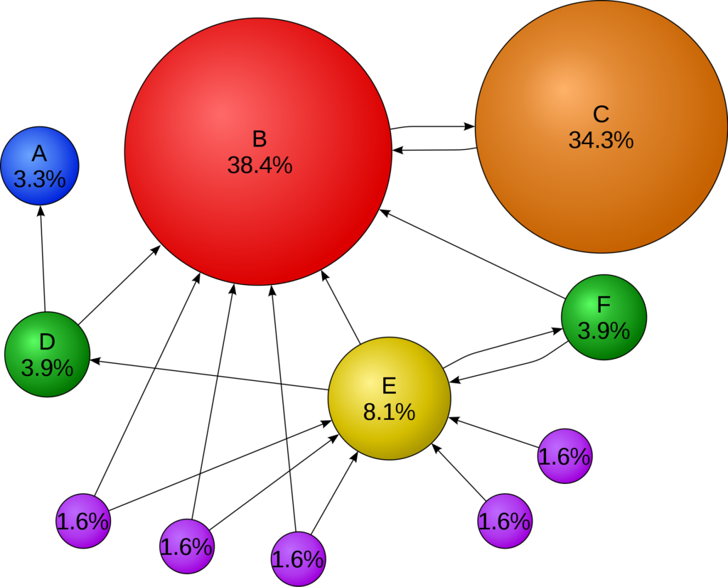
An example of the PageRank distribution for a small internet is shown below. As one would expect, the surfer spends a large part of their time on website B, which has many incoming links. Interestingly, the user spends almost as much of their time on website C, whose only links are to and from B. Under the PageRank model, a website is important if it is linked to by an important website, even if that is the only website linking to it.

Markov Chains in General

Having seen one Markov chain, the PageRank internet surfer, let’s talk about Markov chains in general. A (time-homogeneous) Markov chain consists of two things: a set of states and probabilities for transitioning between states:

Set of states. For this discussion, we limit ourselves to Markov chains which can only exist in finitely many different states. To simplify our discussion, label the possible states using numbers $1,2,\ldots,m$ .
Transition probabilities. The definining property of a (time-homogeneous) Markov chain is that, at any point in time $n$ , if the state is $i$ , the probability of moving to state $j$ is a fixed number $P_{ij}$ . In particular, the probability $P_{ij}$ of moving from $i$ to $j$ does not depend on the time $n$ or the past history of the chain before time $n$ ; only the value of the chain at time $n$ matters.

Denote the state of the Markov chain at times $0,1,2,\ldots$ by $x_0,x_1,x_2,\ldots$ . Note that the states $x_0,x_1,x_2,\ldots$ are random quantities. We can write the Markov chain property using the language of conditional probability:

$\mathbb{P} \{ x_{n+1} = j \mid x_n = i,x_{n-1}=a_{n-1},\ldots,x_0=a_0\} = \mathbb{P}\{x_{n+1} = j \mid x_n = i\} = P_{ij}.$

This equation states that the probability that the system is in state $j$ at time $n+1$ given the entire history of the system depends only on the value $x_n = i$ of the chain at time $n$ . This probability is the transition probability $P_{ij}$ .

Let’s see how the PageRank internet surfer fits into this model:

Set of states. Here, the set of states are the websites, which we label $1,\ldots,m$ .
Transition probabilities. Consider two websites $i$ and $j$ . If $i$ does not have a link to $j$ , then the only way of going from $i$ to $j$ is if the surfer randomly gets bored (probability 15%) and picks website $j$ to visit at random (probability $1/m$ ). Thus,
( $i\not\to j$ ) $P_{ij} = \frac{0.15}{m}.$
Suppose instead that $i$ does link to $j$ and $i$ has $d_i$ outgoing links. Then, in addition to the $0.15/m$ probability computed before, user $i$ has an 85% percent chance of following a link and a $1/d_i$ chance of picking $j$ as that link. Thus,
( $i\to j$ ) $P_{ij} = \frac{0.85}{d_i} + \frac{0.15}{m}.$

Markov Chains and Linear Algebra

For a non-random process $y_0,y_1,y_2,\ldots$ , we can understand the processes evolution by determining its state $y_n$ at every point in time $n$ . Since Markov chains are random processes, it is not enough to track the state $x_n$ of the process at every time $n$ . Rather, we must understand the probability distribution of the state $x_n$ at every point in time $n$ .

It is customary in Markov chain theory to represent a probability distribution on the states $\{1,\ldots,n\}$ by a row vector $\rho^\top$ .¹ The $i$ th entry $\rho_i$ stores the probability that the system is in state $i$ . Naturally, as $\rho^\top$ is a probability distribution, its entries must be nonnegative ( $\rho_i \ge 0$ for every $i$ ) and add to one ( $\sum_{i=1}^n \rho_i = 1$ ).

Let $(\rho^{(0)})^\top, (\rho^{(1)})^\top,\ldots$ denote the probability distributions of the states $x_0,x_1,\ldots$ . It is natural to ask: How are the distributions $(\rho^{(0)})^\top, (\rho^{(1)})^\top,\ldots$ related to each other? Let’s answer this question.

The probability that $x_{n+1}$ is in state $j$ is the $j$ th entry of $\rho^{(n+1)}$ :

$\rho^{(n+1)}_j = \mathbb{P} \{x_{n+1} = j\}$

To compute this probability, we break into cases based on the value of the process at time $n$ : either $x_n = 1$ or $x_n = 2$ or … or $x_n = m$ ; only one of these cases can be true at once. When we have an “or” of random events and these events are mutually exclusive (only can be true at once), then the probabilities add:

$\rho^{(n+1)}_j = \mathbb{P} \{x_{n+1} = j\} = \sum_{i=1}^m \mathbb{P} \{x_{n+1} = j, x_n = i\}.$

Now we use some conditional probability. The probability that $x_{n+1} = j$ and $x_n = i$ is the probability that $x_n = i$ times the probability that $x_{n+1} = j$ conditional on $x_n = i$ . That is,

$\rho^{(n+1)}_j = \sum_{i=1}^m \mathbb{P} \{x_{n+1} = j, x_n = i\} = \sum_{i=1}^m \mathbb{P} \{x_n = i\} \mathbb{P}\{x_{n+1} = j \mid x_n = i\}.$

Now, we can simplify using our definitions. The probability that $x_n = i$ is just $\rho^{(n)}_i$ and the probability of moving from $i$ to $j$ is $P_{ij}$ . Thus, we conclude

$\rho_j^{(n+1)} = \sum_{i=1}^m \rho^{(n)}_i P_{ij} .$

Phrased in the language of linear algebra, we’ve shown

$\left(\rho^{(n+1)}\right)^\top = \left(\rho^{(n)}\right)^\top P \quad \text{for any } n = 0,1,2,\ldots.$

That is, if we view the transition probabilities $P_{ij}$ as comprising an $m\times m$ matrix $P$ , then the distribution at time $n+1$ is obtained by multiplying the distribution at time $n$ by transition matrix $P$ . In particular, if we iterate this result, we obtain that the distribution at time $n$ is given by

$\left(\rho^{(n)}\right)^\top = \left(\rho^{(n-1)}\right)^\top P = \left[\left(\rho^{(n-2)}\right)^\top P\right]P = \left(\rho^{(n-2)}\right)^\top P^2 = \cdots = \left(\rho^{(0)}\right)^\top P^n.$

Thus, the distribution at time $n$ is the distribution at time $0$ multiplied by the $n$ th power of the transition matrix $P$ .

Convergence to Stationarity

Let’s go back to our web surfer again. At time $0$ , we started our surfer at a particular website, say $1$ . As such, the probability distribution² $\rho^{(0)}$ at time $0$ is concentrated just on website $1$ , with no other website having any probability at all. In the first few steps, most of the probability will remain in the vacinity of website $1$ , in the websites linked to by $1$ and the websites linked to by the websites linked to by $1$ and so on. However, as we run the chain long enough, the surfer will have time to widely across the web and the probability distribution will become less and less influenced by the chain’s starting location. This motivates the following definition:

Definition. A Markov chain satisfies the mixing property if the probability distributions $\rho^{(0)}, \rho^{(1)}, \ldots$ converge to a single fixed probability distribution $\pi$ regardless of how the chain is initialized (i.e., independent of the starting distribution $\rho^{(0)}$ ).

The distribution $\pi$ for a mixing Markov chain is known as a stationary distribution because it does not change under the action of $P$ :

(St) $\pi^\top = \pi^\top P.$

To see this, recall the recurrence

$\left(\rho^{(n+1)}\right)^\top = \left(\rho^{(n)}\right)^\top P,$

take the limit as $n\to\infty$ , and observe that both $(\rho^{(n+1)})^\top$ and $(\rho^{(n)})^\top$ converge to $\pi^\top$ .

One of the basic questions in the theory of Markov chains is finding conditions under which the mixing property (or suitable weaker versions of it) hold. To answer this question, we will need the following definition:

A Markov chain is primitive if, after running the chain for some number $n$ steps, the chain has positive probability of moving between any two states. That is,
$\text{There exists $n$ such that, for any $i,j = 1,2,\ldots,m$, } \quad\mathbb{P}\{x_n = j \mid x_0 = i \} = (P^n)_{ij} > 0.$

The fundamental theorem of Markov chains is that primitive chains satisfy the mixing property.

Theorem (fundamental theorem of Markov chains). Every primitive Markov chain is mixing. In particular, there exists one and only probability distribution $\pi$ satisfying the stationary property (St) and the probability distributions $\rho^{(0)},\rho^{(1)},\ldots$ converge to $\pi$ when initialized in any probability distribution $\rho^{(0)}$ . Every entry of $\pi$ is strictly positive.

Let’s see an example of the fundamental theorem with the PageRank surfer. After $n=1$ step, there is at least a $0.15/m > 0$ chance of moving from any website $i$ to any other website $j$ . Thus, the chain is primitive. Consequently, there is a unique stationary distribution $\pi$ , and the surfer will converge to this stationary distribution regardless of which website they start at.

Going Backwards in Time

Often, it is helpful to consider what would happen if we ran a Markov chain backwards in time. To see why this is an interesting idea, suppose you run website $w$ and you’re interested in where your traffic is coming from. One way of achieving this would be to initialize the Markov chain at $w$ and run the chain backwards in time. Rather than asking, “given I’m at $w$ now, where would a user go next?”, you ask “given that I’m at $w$ now, where do I expect to have come from?”

Let’s formalize this notion a little bit. Consider a primitive Markov chain $x_0,x_1,x_2,\ldots$ with stationary distribution $\pi$ . We assume that we initialize this Markov chain in the stationary distribution. That is, we pick $\rho^{(0)} = \pi$ as our initial distribution for $x_0$ . The time-reversed Markov chain $y_0,y_1,\ldots$ is defined as follows: The probability $P^{\rm rev}_{ij}$ of moving from $i$ to $j$ in the time-reversed Markov chain is the probability that I was at state $j$ one step previously given that I’m at state $i$ now:

$\mathbb{P} \{y_1 = j \mid y_0 = i\} = P^{\rm rev}_{ij} = \mathbb{P} \{ x_0 = j \mid x_1 = i \}.$

To get a nice closed form expression for the reversed transition probabilities $P^{\rm rev}_{ij}$ , we can invoke Bayes’ theorem:

(Rev) $P^{\rm rev}_{ij} = \mathbb{P} \{ x_0 = j \mid x_1 = i \} = \frac{\mathbb{P} \{x_0 = j\} \mathbb{P} \{x_1 = i \mid x_0 = j\}}{\mathbb{P} \{x_1 = i\}} = \frac{ \pi_j P_{ji}}{\pi_i}.$

The time-reversed Markov chain can be a strange beast. For the reversed PageRank surfer, for instance, follows links “upstream” traveling from the linked site to the linking site. As such, our hypothetical website owner could get a good sense of where their traffic is coming from by initializing the reversed chain $y_0 = w$ at their website and following the chain one step back.

Reversible Markov Chains

We now have two different Markov chains: the original and its time-reversal. Call a Markov chain reversible if these processes are the same. That is, if the transition probabilities are the same:

$P^{\rm rev}_{ij} = P_{ij} \quad \text{for every } i,j=1,2,\ldots,m.$

Using our formula (Rev) for the reversed transition probability, the reversibility condition can be written more concisely as

$\pi_i P_{ij} = \pi_j P_{ji}.$

This condition is referred to as detailed balance.³ In words, it states that a Markov chain is reversible if, when initialized in the stationary distribution $\pi$ , the flow of probability mass from $i$ to $j$ (that is, $\pi_i P_{ij}$ ) is equal to the flow of probability mass from $j$ to $i$ (that is, $\pi_jP_{ji}$ ).

Many interesting Markov chains are reversible. One class of examples are Markov chain models of physical and chemical processes. Since physical laws like classical and quantum mechanics are reversible under time, so too should we expect Markov chain models built from theories to be reversible.

Not every interesting Markov chain is reversible, however. Indeed, except in special cases, the PageRank Markov chain is not reversible. If $i$ links to $j$ but. $j$ does not link to $i$ , then the flow of mass from $i$ to $j$ will be higher than the flow from $j$ to $i$ .

Before moving on, we note one useful fact about reversible Markov chains. Suppose a reversible, primitive Markov chain satisfies the detailed balance condition with a probability distribution $\sigma$ :

$\sigma_i P_{ij} = \sigma_j P_{ji}.$

Then $\sigma = \pi$ is the stationary distribution of this chain. To see why, we check the stationarity condition $\sigma^\top P = \sigma^\top$ . Indeed, for every $j$ ,

$(\sigma^\top P)_j = \sum_{i=1}^m \sigma_i P_{ij} = \sum_{i=1}^m \sigma_j P_{ji} = \sigma_j.$

The second equality is detailed balance and the third equality is just the condition that the sum of the transition probabilities from $j$ to each $i$ is one. Thus, $\sigma^\top P = \sigma^\top$ and $\sigma$ is a stationary distribution for $P$ . But a primitive chain has only one stationary distribution $\pi$ , so $\sigma = \pi$ .

Markov Chains as Algorithms

Markov chains are an amazingly flexible tool. One use of Markov chains is more scientific: Given a system in the real world, we can model it by a Markov chain. By simulating the chain or by studying its mathematical properties, we can hope to learn about the system we’ve modeled.

Another use of Markov chains is algorithmic. Rather than thinking of the Markov chain as modeling some real-world process, we instead design the Markov chain to serve a computationally useful end. The PageRank surfer is one example. We wanted to rank the importance of websites, so we designed a Markov chain to achieve this task.

One task we can use Markov chains to solve are sampling problems. Suppose we have a complicated probability distribution $\pi$ , and we want a random sample from $\pi$ —that is, a random quantity $y$ such that $\mathbb{P} \{ y = i \} = \pi_i$ for every $i$ . One way to achieve this goal is to design a primitive Markov chain with stationary distribution $\pi$ . Then, we run the chain for a large number of steps $n$ and use $x_n$ as an approximate sample from $\pi$ .

To design a Markov chain with stationary distribution $\pi$ , it is sufficient to generate transition probabilities $P$ such that $\pi$ and $P$ satisfy the detailed balance condition. Then, we are guaranteed that $\pi$ is a stationary distribution for the chain. (We also should check the primitiveness condition, but this is often straightforward.)

Here is an effective way of building a Markov chain to sample from a distribution $\pi$ . Suppose that the chain is in state $i$ at time $n$ , $x_n = i$ . To choose the next state, we begin by sampling $j$ from a proposal distribution $T$ . The proposal distribution $T$ can be almost anything we like, as long as it satisfies three conditions:

Probability distribution. For every $i$ , the transition probabilitie $T_{ij}$ add to one: $\sum_{j=1}^m T_{ij} = 1$ .
Bidirectional. If $T_{ij} > 0$ , then $T_{ji} > 0$ .
Primitive. The transition probabilities $T$ form a primitive Markov chain.

In order to sample from the correct distribution, we can’t just accept every proposal. Rather, given the proposal $i\to j$ , we accept with probability

$\min \left\{ 1 , \frac{\pi_j T_{ji}}{\pi_i T_{ij}} \right\}.$

If we accept the proposal, the next state of our chain is $x_{n+1} = j$ . Otherwise, we stay where we are $x_{n+1} = i$ . This Markov chain is known as a Metropolis–Hastings sampler.

For clarity, we list the steps of the Metropolis–Hastings sampler explicitly:

Initialize the chain in any state $x_0$ and set $n := 0$ .
Draw a proposal $x'$ with from the proposal distribution, $\mathbb{P} \{ x' = j \} = T_{x_nj}$ .
Compute the acceptance probability
$p_{\rm acc} := \min \left\{ 1 , \frac{\pi_j T_{ji}}{\pi_i T_{ij}} \right\}.$
With probability $p_{\rm acc}$ , set $x_{n+1} := x'$ . Otherwise, set $x_{n+1} := x_n$ .
Set $n := n+1$ and go back to step 2.

To check that $\pi$ is a stationary distribution of the Metropolis–Hastings distribution, all we need to do is check detailed balance. Note that the probability $P_{ij}$ of transitioning from $i$ to $j\ne i$ under the Metropolis–Hastings sampler is the proposal probability $T_{ij}$ times the acceptance probability:

$P_{ij} = T_{ij} \cdot \min \left\{ 1 , \frac{\pi_j T_{ji}}{\pi_i T_{ij}} \right\}.$

Detailed balance is confirmed by a short computation⁴

$\pi_i P_{ij} = \pi_i T_{ij} \cdot \min \left\{ 1 , \frac{\pi_j T_{ji}}{\pi_i T_{ij}} \right\} = \min \left\{ \pi_i T_{ij} , \pi_j T_{ji} \right\} = \pi_j P_{ji}.$

Thus the Metropolis–Hastings sampler has $\pi$ as stationary distribution.

Determinatal Point Processes: Diverse Items from a Collection

The uses of Markov chains in science, engineering, math, computer science, and machine learning are vast. I wanted to wrap up with one application that I find particularly neat.

Suppose I run a bakery and I sell $N$ different baked goods. I want to pick out $k$ special items for a display window to lure customers into my store. As a first approach, I might pick my top- $k$ selling items for the window. But I realize that there’s a problem. All of my top sellers are muffins, so all of the items in my display window are muffins. My display window is doing a good job luring in muffin-lovers, but a bad job of enticing lovers of other baked goods. In addition to rating the popularity of each item, I should also promote diversity in the items I select for my shop window.

Here’s a creative solution to my display case problems using linear algebra. Suppose that, rather than just looking at a list of the sales of each item, I define a matrix $A$ for my baked goods. In the $ii$ th entry $A_{ii}$ of my matrix, I write the number of sales for baked good $i$ . I populate the off-diagonal entries $A_{ij}$ of my matrix with a measure of similarity between items $i$ and $j$ .⁵ So if $i$ and $j$ are both muffins, $A_{ij}$ will be large. But if $i$ is a muffin and $j$ is a cookie, then $A_{ij}$ will be small. For mathematical reasons, we require $A$ to be symmetric and positive definite.

To populate my display case, I choose a random subset of $k$ items from my full menu of size $N$ according to the following strange probability distribution: The probability $\pi_S$ of picking items $S = \{s_1,\ldots,s_k\} \subseteq \{1,\ldots,N\}$ is proportional to the determinant of the submatrix $A(S,S)$ . More specifically,

( $k$ -DPP) $\pi_S = \frac{\det A(S,S)}{\sum_{\text{all subsets $T$ of size $k$}} \det A(T,T)}.$

Here, we let $A(S,S)$ denote the $k\times k$ submatrix of $A$ consisting of the entries appearing in rows and columns $s_1,\ldots,s_k$ . Such a random subset is known as a $k$ -determinantal point process ( $k$ -DPP). (See this survey for more about DPPs.)

To see why this makes any sense, let’s consider a simple example of $N = 3$ items and a display case of size $k = 2$ . Suppose I have three items: a pumpkin muffin, a chocolate chip muffin, and an oatmeal raisin cookies. Say the $A$ matrix looks like

$A = \begin{bmatrix} 10 & 9 & 0 \\ 9 & 10 & 0 \\ 0 & 0 & 5 \end{bmatrix}.$

We see that both muffins are equally popular $A_{11} = A_{22} = 10$ and much more popular than the cookie $A_{33} = 5$ . However, the two muffins are similar to each other and thus the corresponding submatrix has small determinant

$\det A(\{1,2\},\{1,2\}) = \det \twobytwo{10}{9}{9}{10} = 19.$

By contrast, if the cookie is disimilar to each muffin and the determinant is higher

$\det A(\{1,3\},\{1,3\}) = \det A(\{2,3\},\{2,3\}) = \det \twobytwo{10}{0}{0}{5} = 50.$

Thus, even though the muffins are more popular overall, choosing our display case from a $2$ -DPP, we have a $(50+50) / (50+50+19) \approx 84\%$ chance of choosing a muffin and a cookie for our display case. It is for this reason that we can say that a $k$ -DPP preferentially selects for diverse items.

Is sampling from a $k$ -DPP the best way of picking $k$ items for my display case? How does it compare to other possible methods?⁶ These are interesting questions for another time. For now, let us focus our attention on a different question: How would you sample from a $k$ -DPP?

Determinantal Point Process by Markov Chains

Sampling from a $k$ -DPP is a hard computational problem. Indeed, there are ${N \choose k}$ possible $k$ -element subspaces of a set of $N$ items. The number of possibilities gets large fast. If I have $N = 100$ items and want to pick $k = 10$ of them, there are already over 10 trillion possible combinations.

Markov chains offer one compelling way of sampling a $k$ -DPP. First, we need a proposal distribution. Let’s choose the simplest one we can think of:

Proposal for $k$ -DPP sampling. Suppose our current set of $k$ items is $S = \{s_1,\ldots,s_k\}$ . To generate a proposal, choose a uniformly random element $s_{\rm old}$ out of $S$ and a uniformly random element $s_{\rm new}$ out of $\{1,\ldots,N\}$ without $S$ . Propose $S'$ obtained from $S$ by replacing $s_{\rm old}$ with $s_{\rm new}$ (i.e., $S' = S \cup \{s_{\rm new}\} \setminus \{s_{\rm old}\}$ ).

Now, we need to compute the Metropolis–Hastings acceptance probability

$p_{\rm acc} = \min \left\{ 1 , \frac{\pi_{S'} T_{S'S}}{\pi_{S} T_{SS'}} \right\}.$

For $S$ and $S'$ which differ only by the addition of one element and the removal of another, the proposal probabilities $T_{S'S}$ and $T_{SS'}$ are both equal to $1/(kN)$ , $T_{S'S} = T_{SS'} = 1/(kN)$ . Using the formula for the probability $\pi_S$ of drawing $S$ from a $k$ -DPP, we compute that

$\frac{\pi_{S'}}{\pi_S} = \frac{\det A(S',S')}{\det A(S,S)}.$

Thus, the Metropolis–Hastings acceptance probability is just a ratio of determinants:

(Acc) $p_{\rm acc} = \min \left\{ 1 , \frac{\pi_{S'} T_{S'S}}{\pi_{S} T_{SS'}} \right\} = \min \left\{ 1, \frac{\det A(S',S')}{\det A(S,S)} \right\}.$

And we’re done. Let’s summarize our sampling algorithm:

Choose an initial set $S_0$ arbitrarily and set $n := 0$ .
Draw $s_{\rm old}$ uniformly at random from $S_n$ .
Draw $s_{\rm new}$ uniformly at random from $\{1,\ldots,N\} \setminus S_n$ .
Set $S' := S_n \cup \{s_{\rm new}\} \setminus \{s_{\rm old}\}$ .
With probability $p_{\rm acc}$ defined in (Acc), accept and set $S_{n+1} := S'$ . Otherwise, set $S_{n+1} := S_n$ .
Set $n := n+1$ and go to step 2.

This is a remarkably simple algorithm to sample from a complicated distribution. And its fairly efficient as well. Analysis by Anari, Oveis Gharan, and Rezaei shows that, when you pick a good enough initial set $S_0$ , this sampling algorithm produces approximate samples from a $k$ -DPP in roughly $Nk^2$ steps.⁷ Remarkably, if $k$ is much smaller than $N$ , this Markov chain-based algorithm samples from a $k$ -DPP without even looking at all $N^2$ entries of the matrix $A$ !

Upshot. Markov chains are a simple and general model for a state evolving randomly in time. Under mild conditions, Markov chains converge to a stationary distribution: In the limit of a large number of steps, the state of the system become randomly distributed in a way independent of how it was initialized. We can use Markov chains as algorithms to approximately sample from challenging distributions.

Big Ideas in Applied Math: Concentration Inequalities

August 2, 2022 by Ethan N. Epperly 3 Comments

This post is about randomized algorithms for problems in computational science and a powerful set of tools, known as concentration inequalities, which can be used to analyze why they work. I’ve discussed why randomization can help in solving computational problems in a previous post; this post continues this discussion by presenting an example of a computational problem where, somewhat surprisingly, a randomized algorithm proves effective. We shall then use concentration inequalities to analyze why this method works.

Triangle Counting

Let’s begin our discussion of concentration inequalities by means of an extended example. Consider the following question: How many triangles are there in the Facebook network? That is, how many trios of people are there who are all mutual friends? While seemingly silly at first sight, this is actually a natural and meaningful question about the structure of the Facebook social network and is related to similar questions such as “How likely are two friends of a person to also be friends with each other?”

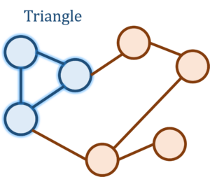
If there are $n$ people on the Facebook graph, then the natural algorithm of iterating over all ${n \choose 3} \approx n^3/6$ triplets and checking whether they form a triangle is far too computationally costly for the billions of Facebook accounts. Somehow, we want to do much faster than this, and to achieve this speed we would be willing to settle for an estimate of the triangle count up to some error.

There are many approaches to this problem, but let’s describe a particularly surprising algorithm. Let $A$ be an $n\times n$ matrix where the $ij$ th entry of $A$ is $1$ if users $i$ and $j$ are friends and $0$ otherwise¹; this matrix is called the adjacency matrix of the Facebook graph. A fact from graph theory is that the $ij$ th entry of the cube $A^3$ of the matrix $A$ counts the number of paths from user $i$ to user $j$ of length three.² In particular, the $ii$ th entry of $A^3$ denotes the number of paths from $i$ to itself of length $3$ , which is twice the number of triangles incident on $i$ . (The paths $i\to j \to k \to i$ and $i\to k \to j\to i$ are both counted as paths of length 3 for a triangle consisting of $i$ , $j$ , and $k$ .) Therefore, the trace of $A^3$ , equal to the sum of its diagonal entries, is six times the number of triangles: The $ii$ th entry of $A^3$ is twice the number of triangles incident on $i$ and each triangle $(i,j,k)$ is counted thrice in the $ii$ th, $jj$ th, and $kk$ th entries of $A^3$ . In summary, we have

$\begin{equation*} \mbox{\# triangles} = \frac{1}{6} \operatorname{tr} A^3. \end{equation*}$

Therefore, the triangle counting problem is equivalent to computing the trace of $A^3$ . Unfortunately, the problem of computing $A^3$ is, in general, very computationally costly. Therefore, we seek ways of estimating the trace of a matrix without forming it.

Randomized Trace Estimation

Motivated by the triangle counting problem from the previous section, we consider the problem of estimating the trace of a matrix $M$ . We assume that we only have access to the matrix $M$ through matrix–vector products; that is, we can efficiently compute $Mx$ for a vector $x$ . For instance, in the previous example, the Facebook graph has many fewer friend relations (edges) $m$ than the maximum possible amount of ${n\choose 2} \approx n^2/2$ . Therefore, the matrix $A$ is sparse; in particular, matrix–vector multiplications with $A$ can be computed in around $m$ operations. To compute matrix–vector products $Mx$ with $M = A^3$ , we simply compute matrix–vector products with $A$ three times, $x \mapsto Ax \mapsto A(Ax) \mapsto A(A(Ax)) = A^3x$ .

Here’s a very nifty idea to estimate the trace of $M$ using only matrix–vector products, originally due to Didier A. Girard and Michael F. Hutchinson. Choose $x$ to be a random vector whose entries are independent $\pm 1$ -values, where each value $+1$ and $-1$ occurs with equal $1/2$ probability. Then if one forms the expression $x^\top M x = \sum_{i,j=1}^n M_{ij} x_i x_j$ . Since the entries of $x_i$ and $x_j$ are independent, the expectation of $x_ix_j$ is $0$ for $i\ne j$ and $1$ for $i = j$ . Consequently, by linearity of expectation, the expected value of $x^\top M x$ is

$\begin{equation*} \mathbb{E} \, x^\top M x = \sum_{i,j=1}^n M_{ij} \mathbb{E} [x_ix_j] = \sum_{i = 1}^n M_{ii} = \operatorname{tr}(M). \end{equation*}$

The average value of $x^\top M x$ is equal to the trace of $M$ ! In the language of statistics, we might say that $x^\top M x$ is an unbiased estimator for $\operatorname{tr}(M)$ . Thus, the efficiently computable quantity $x^\top M x$ can serve as a (crude) estimate for $\operatorname{tr}(M)$ .

While the expectation of $x^\top Mx$ equals $\operatorname{tr}(M)$ , any random realization of $x^\top M x$ can deviate from $\operatorname{tr}(M)$ by a non-neligible amount. Thus, to reduce the variability of the estimator $x^\top M x$ , it is appropriate to take an average of multiple copies of this random estimate. Specifically, we draw $k$ random vectors with independent random $\pm 1$ entries $x_1,\ldots,x_k$ and compute the averaged trace estimator

(1) $\begin{equation*} T_k := \frac{1}{k} \sum_{j=1}^k x_j^\top M x_j^{\vphantom{\top}}. \end{equation*}$

The $k$ -sample trace estimator $T_k$ remains an unbiased estimator for $\operatorname{tr}(M)$ , $\mathbb{E}\, T_k = \operatorname{tr}(M)$ , but with reduced variability. Quantitatively, the variance of $T_k$ is $k$ times smaller than the single-sample estimator $x^\top M x$ :

(2) $\begin{equation*} \operatorname{Var}(T_k) = \frac{1}{k} \operatorname{Var}(x^\top M x). \end{equation*}$

The Girard–Hutchinson trace estimator gives a natural way of estimating the trace of the matrix $M$ , a task which might otherwise be hard without randomness.³ For the trace estimator to be a useful tool, an important question remains: How many samples $k$ are needed to compute $\operatorname{tr}(M)$ to a given accuracy? Concentration inequalities answer questions of this nature.

Concentration Inequalities

A concentration inequality provides a bound on the probability a random quantity is significantly larger or smaller than its typical value. Concentration inequalities are useful because they allow us to prove statements like “With at least 99% probability, the randomized trace estimator with 100 samples produces an approximation of the trace which is accurate up to error no larger than $0.001$ .” In other words, concentration inequalities can provide quantitative estimates of the likely size of the error when a randomized algorithm is executed.

In this section, we shall introduce a handful of useful concentration inequalities, which we will apply to the randomized trace estimator in the next section. We’ll then discuss how these and other concentration inequalities can be derived in the following section.

Markov’s Inequality

Markov’s inequality is the most fundamental concentration inequality. When used directly, it is a blunt instrument, requiring little insight to use and producing a crude but sometimes useful estimate. However, as we shall see later, all of the sophisticated concentration inequalities that will follow in this post can be derived from a careful use of Markov’s inequality.

The wide utility of Markov’s inequality is a consequence of the minimal assumptions needed for its use. Let $X$ be any nonnegative random variable. Markov’s inequality states that the probability that $X$ exceeds a level $t > 0$ is bounded by the expected value of $X$ over $t$ . In equations, we have

(3) $\begin{equation*} \mathbb{P} \left\{ X \ge t \right\} \le \frac{\mathbb{E} \, X}{t}. \end{equation*}$

We stress the fact that we make no assumptions on how the random quantity $X$ is generated other than that $X$ is nonnegative.

As a short example of Markov’s inequality, suppose we have a randomized algorithm which takes one second on average to run. Markov’s inequality then shows that the probability the algorithm takes more than 100 seconds to run is at most $1/100 = 1\%$ . This small example shows both the power and the limitation of Markov’s inequality. On the negative side, our analysis suggests that we might have to wait as much as 100 times the average runtime for the algorithm to complete running with 99% probability; this large huge multiple of 100 seems quite pessimistic. On the other hand, we needed no information whatsoever about how the algorithm works to do this analysis. In general, Markov’s inequality cannot be improved without more assumptions on the random variable $X$ .⁴

Chebyshev’s Inequality and Averages

The variance of a random variable describes the expected size of a random variable’s deviation from its expected value. As such, we would expect that the variance should provide a bound on the probability a random variable is far from its expectation. This intuition indeed is correct and is manifested by Chebyshev’s inequality. Let $X$ be a random variable (with finite expected value) and $t > 0$ . Chebyshev’s inequality states that the probability that $X$ deviates from its expected value by more than $t$ is at most $\operatorname{Var}(X)/t^2$ :

(4) $\begin{equation*} \mathbb{P} \left\{ \left| X - \mathbb{E} \, X \right| \ge t \right\} \le \frac{\operatorname{Var}(X)}{t^2}. \end{equation*}$

Chebyshev’s inequality is frequently applied to sums or averages of independent random quantities. Suppose $X_1,\ldots,X_n$ are independent and identically distributed random variables with mean $\mu$ and variance $\sigma^2$ and let $\overline{X}$ denote the average

$\begin{equation*} \overline{X} = \frac{X_1 + \cdots + X_n}{n}. \end{equation*}$

Since the random variables $X_1,\ldots,X_n$ are independent,⁵ the properties of variance entail that

$\begin{equation*} \operatorname{Var}(\overline{X}) = \operatorname{Var}\left( \frac{1}{n} X_1 + \cdots + \frac{1}{n} X_n \right) = \frac{1}{n^2} \operatorname{Var}(X_1) + \cdots + \frac{1}{n^2} \operatorname{Var}(X_n) = \frac{\sigma^2}{n}, \end{equation*}$

where we use the fact that $\operatorname{Var}(X_1) = \cdots = \operatorname{Var}(X_n) = \sigma^2$ . Therefore, by Chebyshev’s inequality,

(5) $\begin{equation*} \mathbb{P} \left\{ \left| \overline{X} - \mu \right| \ge t \right\} \le \frac{\sigma^2}{nt^2}. \end{equation*}$

Suppose we want to estimate the mean $\mu$ by $\overline{X}$ up to error $\epsilon$ and are willing to tolerate a failure probability of $\delta$ . Then setting the right-hand side of (5) to $\delta$ , Chebyshev’s inequality suggests that we need at most

(6) $\begin{equation*} n = \sigma^2\cdot \frac{1/\delta}{\epsilon^2} \end{equation*}$

samples to achieve this goal.

Exponential Concentration: Hoeffding and Bernstein

How happy should we be with the result (6) of applying Chebyshev’s inequality the average $\overline{X}$ ? The central limit theorem suggests that $\overline{X}$ should be approximately normally distributed with mean $\mu$ and variance $\sigma^2/n$ . Normal random variables have an exponentially small probability of being more than a few standard deviations above their mean, so it is natural to expect this should be true of $\overline{X}$ as well. Specifically, we expect a bound roughly like

(7) $\begin{equation*} \mathbb{P} \left\{ \left| \overline{X} - \mu \right| \ge t \right\} \stackrel{?}{\lessapprox} \exp\left(-\frac{nt^2}{2\sigma^2}\right). \end{equation*}$

Unfortunately, we don’t have a general result quite this nice without additional assumptions, but there are a diverse array of exponential concentration inequalities available which are quite useful in analyzing sums (or averages) of independent random variables that appear in applications.

Hoeffding’s inequality is one such bound. Let $X_1,\ldots,X_n$ be independent (but not necessarily identically distributed) random variables and consider the average $\overline{X} = (X_1 + \cdots + X_n)/n$ . Hoeffding’s inequality makes the assumption that the summands are bounded, say within an interval $[a,b]$ .⁶ Hoeffding’s inequality then states that

(8) $\begin{equation*} \mathbb{P}\left\{ \left|\overline{X} - \mathbb{E} \, \overline{X}\right| \ge t \right\} \le 2 \exp\left( -\frac{2nt^2}{(b-a)^2} \right). \end{equation*}$

Hoeffding’s inequality is quite similar to the ideal concentration result (7) except with the variance $\sigma^2 = n\operatorname{Var}(\overline{X})$ replaced by the potentially much larger quantity⁷ $(b-a)^2/4$ .

Bernstein’s inequality fixes this deficit in Hoeffding’s inequality at a small cost. Now, instead of assuming $X_1,\ldots,X_n$ are bounded within the interval $[a,b]$ , we make the alternate boundedness assumption $|X_i - \mathbb{E}\, X_i| \le B$ for every $1\le i\le n$ . We continue to denote $\sigma^2 = n\operatorname{Var}(\overline{X})$ so that if $X_1,\ldots,X_n$ are identically distributed, $\sigma^2$ denotes the variance of each of $X_1,\ldots,X_n$ . Bernstein’s inequality states that

(9) $\begin{equation*} \mathbb{P}\left\{ \left|\overline{X} - \mathbb{E} \, \overline{X}\right| \ge t \right\} \le 2 \exp\left( -\frac{nt^2/2}{\sigma^2 + Bt/3} \right). \end{equation*}$

For small values of $t$ , Bernstein’s inequality yields exactly the kind of concentration that we would hope for from our central limit theorem heuristic (7). However, for large values of $t$ , we have

$\begin{equation*} \mathbb{P}\left\{ \left|\overline{X} - \mathbb{E} \, \overline{X}\right| \ge t \right\} \stackrel{\mbox{large $t$}}{\lessapprox} 2 \exp\left( -\frac{3nt}{2B} \right), \end{equation*}$

which is exponentially small in $t$ rather than $t^2$ . We conclude that Bernstein’s inequality provides sharper bounds then Hoeffding’s inequality for smaller values of $t$ but weaker bounds for larger values of $t$ .

Chebyshev vs. Hoeffding vs. Bernstein

Let’s return to the situation where we seek to estimate the mean $\mu$ of independent and identically distributed random variables $X_1,\ldots,X_n$ each with variance $\sigma^2$ by using the averaged value $\overline{X} = (X_1 + \cdots + X_n)/n$ . Our goal is to bound how many samples $n$ we need to estimate $\mu$ up to error $\epsilon$ , $| \overline{X} - \mu | \le \epsilon$ , except with failure probability at most $\delta$ . Using Chebyshev’s inequality, we showed that (see (7))

$\begin{equation*} n \ge \sigma^2\cdot \frac{1/\delta}{\epsilon^2} \mbox{ suffices}. \end{equation*}$

Now, let’s try using Hoeffding’s inequality. Suppose that $X_1,\ldots,X_n$ are bounded in the interval $[a,b]$ . Then Hoeffding’s inequality (8) shows that

$\begin{equation*} n \ge \frac{(b-a)^2}{4}\cdot \frac{2\log(2/\delta)}{\epsilon^2} \mbox{ suffices}. \end{equation*}$

Bernstein’s inequality states that if $X_1,\ldots,X_n$ lie in the interval $[\mu-B,\mu+B]$ for every $1\le i \le n$ , then

(10) $\begin{equation*} n \ge \sigma^2 \cdot \frac{2\log(2/\delta)}{\epsilon^2} + B\cdot \frac{2/3\cdot\log(2/\delta)}{\epsilon} \mbox{ suffices}. \end{equation*}$

Hoeffding’s and Bernstein’s inequality show that we need $n$ roughly proportional to $\tfrac{\log(1/\delta)}{\epsilon^2}$ samples are needed rather than proportional to $\tfrac{1/\delta}{\epsilon^2}$ . The fact that we need proportional to $1/\epsilon^2$ samples to achieve error $\epsilon$ is a consequence of the central limit theorem and is something we would not be able to improve with any concentration inequality. What exponential concentration inequalities allow us to do is to improve the dependence on the failure probability from proportional to $1/\delta$ to $\log(1/\delta)$ , which is a huge improvement.

Hoeffding’s and Bernstein’s inequalities both have a small drawback. For Hoeffding’s inequality, the constant of proportionality is $(b-a)^2/4$ rather than the true variance $\sigma^2$ of the summands. Bernstein’s inequality gives us the “correct” constant of proportionality $\sigma^2$ but adds a second term proportional to $\tfrac{\log(1/\delta)}{\epsilon}$ ; for small values of $\epsilon$ , this term is dominated by the term proportional to $\tfrac{\log(1/\delta)}{\epsilon^2}$ but the second term can be relevant for larger values of $\epsilon$ .

There are a panoply of additional concentration inequalities than the few we’ve mentioned. We give a selected overview in the following optional section.

Other Concentration Inequalities

There are a handful more exponential concentration inequalities for sums of independent random variables such as Chernoff’s inequality (very useful for somes of bounded, positive random variables) and Bennett’s inequality. There are also generalizations of Hoeffding’s, Chernoff’s, and Bernstein’s inequalities for unbounded random variables with subgaussian and subexponential tail decay; these results are documented in Chapter 2 of Roman Vershynin’s excellent book High-Dimensional Probability.

One can also generalize concentration inequalities to so-called martingale sequences, which can be very useful for analyzing adaptive algorithms. These inequalities can often have the advantage of bounding the probability that a martingale sequence ever deviates by some amount from its applications; these results are called maximal inequalities. Maximal analogs of Markov’s and Chebyshev’s inequalities are given by Ville’s inequality and Doob’s inequality. Exponential concentration inequalities include the Hoeffding–Azuma inequality and Freedman’s inequality.

Finally, we note that there are many concentration inequalities for functions of independent random variables other than sums, usually under the assumption that the function is Lipschitz continuous. There are exponential concentration inequalities for functions with “bounded differences”, functions of Gaussian random variables, and convex functions of bounded random variables. References for these results include Chapters 3 and 4 of the lecture notes Probability in High Dimension by Ramon van Handel and the comprehensive monograph Concentration Inequalities by Stéphane Boucheron, Gábor Lugosi, and Pascal Massart.

Analysis of Randomized Trace Estimation

Let us apply some of the concentration inequalities we introduced in last section to analyze the randomized trace estimator. Our goal is not to provide the best possible analysis of the trace estimator,⁸ but to demonstrate how the general concentration inequalities we’ve developed can be useful “out of the box” in analyzing algorithms.

In order to apply Chebyshev’s and Berstein’s inequalities, we shall need to compute or bound the variance of the single-sample trace estimtor $x^\top Mx$ , where $x$ is a random vector of independent $\pm 1$ -values. This is a straightforward task using properties of the variance:

$\begin{equation*} \operatorname{Var}(x^\top M x) = \operatorname{Var}\left( 2\sum_{i< j} M_{ij} x_i x_j \right) = 4\sum_{i\ne j, \: k\ne \ell} M_{ij} M_{k\ell} \operatorname{Cov}(x_ix_j,x_kx_\ell) = 4\sum_{i < j} M_{ij}^2 \le 2 \|M\|_{\rm F}^2 \end{equation*}$

Here, $\operatorname{Cov}$ is the covariance and $\|\cdot\|_{\rm F}$ is the matrix Frobenius norm. Chebyshev’s inequality (5), then gives

$\begin{equation*} \mathbb{P} \left\{ \left|T_k - \operatorname{tr}(M)\right| \ge t \right\} \le \frac{2\|M\|_{\rm F}^2}{kt^2}. \end{equation*}$

Let’s now try applying an exponential concentration inequality. We shall use Bernstein’s inequality, for which we need to bound $|x^\top M x - \operatorname{tr}(M)|$ . By the Courant–Fischer minimax principle, we know that $x^\top M x$ is between $\lambda_{\rm min}(M) \cdot \|x\|^2$ and $\lambda_{\rm max} (M)\cdot\|x\|^2$ where $\lambda_{\rm min}(M)$ and $\lambda_{\rm max}(M)$ are the smallest and largest eigenvalues of $M$ and $\|x\|$ is the Euclidean norm of the vector $x$ . Since all the entries of $x$ have absolute value $1$ , we have $\|x\| = \sqrt{n}$ so $x^\top M x$ is between $n\lambda_{\rm min}(M)$ and $n\lambda_{\rm max}(M)$ . Since the trace equals the sum of the eigenvalues of $M$ , $\operatorname{tr}(M)$ is also between $n\lambda_{\rm min}(M)$ and $n\lambda_{\rm max}(M)$ . Therefore,

$\begin{equation*} \left| x^\top M x - \operatorname{tr}(M) \right| \le n \left( \lambda_{\rm max}(M) - \lambda_{\rm min}(M)\right) \le 2 n \|M\|, \end{equation*}$

where $\|\cdot\|$ denotes the matrix spectral norm. Therefore, by Bernstein’s inequality (9), we have

$\begin{equation*} \mathbb{P} \left\{ \left| T_k - \operatorname{tr}(M) \right| \ge t \right\} \le 2\exp\left( -\frac{kt^2}{4\|M\|_{\rm F}^2 + 4/3\cdot tn\|M\|} \right). \end{equation*}$

In particular, (10) shows that

$\begin{equation*} k \ge \left( \frac{4\|M\|_{\rm F}^2}{\epsilon^2} + \frac{4n\|M\|}{3\epsilon} \right) \log \left(\frac{2}{\delta} \right) \end{equation*}$

samples suffice to estimate $\operatorname{tr}(M)$ to error $\epsilon$ with failure probability at most $\delta$ . Concentration inequalities easily furnish estimates for the number of samples needed for the randomized trace estimator.

We have now accomplished our main goal of using concentration inequalities to analyze the randomized trace estimator, which in turn can be used to solve the triangle counting problem. We leave some additional comments on trace estimation and triangle counting in the following bonus section.

More on Trace Estimation and Triangle Counting

To really complete the analysis of the trace estimator in an application (e.g., triangle counting), we would need to obtain bounds on $\|M\|_{\rm F}$ and $\|M\|$ . Since we often don’t know good bounds for $\|M\|_{\rm F}$ and $\|M \|$ , one should really use the trace estimator together with an a posteriori error estimates for the trace estimator, which provide a confidence interval for the trace rather than a point estimate; see sections 4.5 and 4.6 in this survey for details.

One can improve on the Girard–Hutchinson trace estimator by using a variance reduction technique. One such variance reduction technique was recently proposed under the name Hutch++, extending ideas by Arjun Singh Gambhir, Andreas Stathopoulos, and Kostas Orginos and Lin Lin. In effect, these techniques improve the number of samples $k$ needed to estimate the trace of a positive semidefinite matrix $A$ to relative error $\epsilon$ to proportional to $1/\epsilon$ down from $1/\epsilon^2$ .

Several algorithms have been proposed for triangle counting, many of them randomized. This survey gives a comparison of different methods for the triangle counting problem, and also describes more motivation and applications for the problem.

Deriving Concentration Inequalities

Having introduced concentration inequalities and applied them to the randomized trace estimator, we now turn to the question of how to derive concentration inequalities. Learning how to derive concentration inequalities is more than a matter of mathematical completeness since one can often obtain better results by “hand-crafting” a concentration inequality for a particular application rather than applying a known concentration inequality. (Though standard concentration inequalities like Hoeffding’s and Bernstein’s often give perfectly adequate answers with much less work.)

Markov’s Inequality

At the most fundamental level, concentration inequalities require us to bound a probability by an expectation. In achieving this goal, we shall make a simple observation: The probability that $X$ is larger than or equal to $t$ is the expectation of a random variable $\mathbf{1}_{[t,\infty)}(X)$ .⁹ Here, $\mathbf{1}_{[t,\infty)}(\cdot)$ is an indicator function which outputs one if its input is larger than or equal to $t$ and zero otherwise.

As promised, the probability $X$ is larger than $t$ is the expectation of $\mathbf{1}_{[t,\infty)}(X)$ :

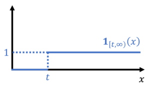
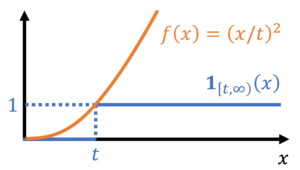
(11) $\begin{equation*} \mathbb{P}\{X \ge t \} = \mathbb{E}[\mathbf{1}_{[t,\infty)}(X)]. \end{equation*}$

We can now obtain bounds on the probability that $X\ge t$ by bounding its corresponding indicator function. In particular, we have the inequality

(12) $\begin{equation*} \mathbf{1}_{[t,\infty)}(x) \le \frac{x}{t} \mbox{ for every } x\ge 0. \end{equation*}$

Since $X$ is nonnegative, combining equations (11) and (12) gives Markov’s inequality:

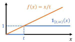
$\begin{equation*} \mathbb{P}\{ X \ge t \} = \mathbb{E}[\mathbf{1}_{[t,\infty)}(X)] \le \mathbb{E} \left[ \frac{X}{t} \right] = \frac{\mathbb{E} X}{t}. \end{equation*}$

Chebyshev’s Inequality

Before we get to Chebyshev’s inequality proper, let’s think about how we can push Markov’s inequality further. Suppose we find a bound on the indicator function $\mathbf{1}_{[t,\infty)}(\cdot)$ of the form

(13) $\begin{equation*} \mathbf{1}_{[t,\infty)}(x) \le f(x) \mbox{ for all } x\ge 0. \end{equation*}$

A bound of this form immediately to bounds on $\mathbb{P} \{X \ge t\}$ by (11). To obtain sharp and useful bounds on $\mathbb{P}\{X\ge t\}$ we seek bounding functions $f(\cdot)$ in (13) with three properties:

For $x\in[0, t)$ , $f(x)$ should be close to zero,
For $x\in [t,\infty)$ , $f(x)$ should be close to one, and
We need $\mathbb{E} \, f(X)$ to be easily computable or boundable.

These three objectives are in tension with each other. To meet criterion 3, we must restrict our attention to pedestrian functions $f(\cdot)$ such as powers $f(x) = (x/t)^\theta$ or exponentials $f(x) = \exp(\theta (x-t))$ for which we have hopes of computing or bounding $\mathbb{E} \, f(X)$ for random variables $X$ we encounter in practical applications. But these candidate functions $f(\cdot)$ have the undesirable property that making the function smaller on $[0, t)$ (by increasing $\theta$ ) to meet point 1 makes the function larger on $(t,\infty)$ , detracting from our ability to achieve point 2. We shall eventually come up with a best-possible resolution to this dilemma by formulating this as an optimization problem to determine the best choice of the parameter $\theta > 0$ to obtain the best possible candidate function of the given form.

Before we get ahead of ourselves, let us use a specific choice for $f(\cdot)$ different than we used to prove Markov’s inequality. We readily verify that $f(x) = (x/t)^2$ satisfies the bound (13), and thus by (12),

(14) $\begin{equation*} \mathbb{P} \{ X \ge t \} \le \mathbb{E} \left( \frac{X}{t} \right)^2 = \frac{\mathbb{E} X^2}{t^2}. \end{equation*}$

This inequality holds for any nonnegative random variable $X$ . In particular, now consider a random variable $X$ which we do not assume to be nonnegative. Then $X$ ‘s deviation from its expectation, $|X-\mathbb{E} X|$ , is a nonnegative random variable. Thus applying (14) gives

$\begin{equation*}\mathbb{P} \{ |X - \mathbb{E} X| \ge t \} \le \frac{\mathbb{E} | X - \mathbb{E} X|^2}{t^2} = \frac{\operatorname{Var}(X)}{t^2}. \end{equation*}$

We have derived Chebyshev’s inequality! Alternatively, one can derive Chebyshev’s inequality by noting that $|X-\mathbb{E} X| \ge t$ if, and only if, $|X-\mathbb{E} X|^2 \ge t^2$ . Therefore, by Markov’s inequality,

$\begin{equation*} \mathbb{P} \{ |X - \mathbb{E} X| \ge t \} = \mathbb{P} \{ |X - \mathbb{E} X|^2 \ge t^2 \} \le \frac{\mathbb{E} | X - \mathbb{E} X|^2}{t^2} = \frac{\operatorname{Var}(X)}{t^2}. \end{equation*}$

The Laplace Transform Method

We shall now realize the plan outlined earlier where we shall choose an optimal bounding function $f(\cdot)$ from the family of exponential functions $f(x) = \exp(\theta(x-t))$ , where $\theta > 0$ is a parameter which we shall optimize over. This method shall allow us to derive exponential concentration inequalities like Hoeffding’s and Bernstein’s. Note that the exponential function $f(x) = \exp(\theta(x-t))$ bounds the indicator function $\mathbf{1}_{[t,\infty)}(\cdot)$ for all real numbers $x$ , so we shall no longer require the random variable $X$ to be nonnegative. Therefore, by (11),

(15) $\begin{equation*} \mathbb{P} \{ X \ge t \} \le \mathbb{E} \exp\left(\theta (X-t)\right) = \exp(-\theta t) \,\mathbb{E} \exp(\theta X) = \exp\left(-\theta t + \log \mathbb{E} \exp(\theta X) \right). \end{equation*}$

The functions

$\begin{equation*} m_X(\theta) = \mathbb{E} \exp(\theta X), \quad \xi_X(\theta) = \log \mathbb{E} \exp(\theta X) = \log m_X(\theta) \end{equation*}$

are known as the moment generating function and cumulant generating function of the random variable $X$ .¹⁰ With these notations, (15) can be written

(16) $\begin{equation*} \mathbb{P} \{ X \ge t \} \le\exp(-\theta t) m_X(\theta) = \exp\left(-\theta t + \xi_X(\theta) \right). \end{equation*}$

The moment generating function coincides with the Laplace transform $\mathbb{E} \exp(-\theta X) = m_X(-\theta)$ up to the sign of the parameter $\theta$ , so one name for this approach to deriving concentration inequalities is the Laplace transform method. (This method is also known as the Cramér–Chernoff method.)

The cumulant generating function has an important property for deriving concentration inequalities for sums or averages of independent random variables: If $X_1,\ldots,X_n$ are independent random variables, than the cumulant generating function is additive:¹¹

(17) $\begin{equation*} \xi_{X_1 + \cdots + X_n}(\theta) = \xi_{X_1}(\theta) + \cdots + \xi_{X_n}(\theta). \end{equation*}$

Proving Hoeffding’s Inequality

For us to use the Laplace transform method, we need to either compute or bound the cumulant generating function. Since we are interested in general concentration inequalities which hold under minimal assumptions such as boundedness, we opt for the latter. Suppose $a\le X \le b$ and consider the cumulant generating function of $Y:=X-\mathbb{E}X$ . Then one can show the cumulant generating function bound¹²

(18) $\begin{equation*} \xi_Y(\theta) \le \frac{1}{8} \theta^2(b-a)^2. \end{equation*}$

Using the additivity of the cumulant generating function (17), we obtain the bound

$\begin{equation*} \xi_{\overline{X} - \mathbb{E} \overline{X}}(\theta) = \xi_{X_1/n- \mathbb{E}X_1/n}(\theta) + \cdots + \xi_{X_n/n- \mathbb{E}X_n/n}(\theta) \le \frac{1}{n} \cdot \frac{1}{8} \theta^2(b-a)^2. \end{equation*}$

Plugging this into the probability bound (16), we obtain the concentration bound

(19) $\begin{equation*} \mathbb{P} \left\{ \overline{X} - \mathbb{E} \overline{X} \ge t \right\} \le \exp \left( - \theta t +\frac{1}{n} \cdot \frac{1}{8} \theta^2(b-a)^2 \right). \end{equation*}$

We want to obtain the smallest possible upper bound on this probability, so it behooves us to pick the value of $\theta > 0$ which makes the right-hand side of this inequality as small as possible. To do this, we differentiate the contents of the exponential and set to zero, obtaining

$\begin{equation*} \frac{\mathrm{d}}{\mathrm{d} \theta} \left( - \theta t + \frac{1}{n} \cdot \frac{1}{8} \theta^2(b-a)^2\right) = - t + \frac{1}{n} \cdot \frac{1}{4} (b-a)^2 \theta = 0\implies \theta = \frac{4nt}{(b-a)^2} \end{equation*}$

Plugging this value for $\theta$ into the bound (19) gives A bound for $\overline{X}$ being larger than $\mathbb{E}\overline{X} + t$ :

(20) $\begin{equation*} \mathbb{P} \left\{ \overline{X} - \mathbb{E} \overline{X} \ge t \right\} \le \exp \left( - \frac{2nt^2}{(b-a)^2} \right). \end{equation*}$

To get the bound on $\overline{X}$ being smaller than $\mathbb{E}\overline{X} - t$ , we can apply a small trick. If we apply (20) to the summands $-X_1,-X_2,\ldots,-X_n$ instead of $X_1,\ldots,X_n$ , we obtain the bounds

(21) $\begin{equation*} \mathbb{P} \left\{ \overline{X} - \mathbb{E} \overline{X} \le -t \right\} \le \exp \left( - \frac{2nt^2}{(b-a)^2} \right). \end{equation*}$

We can now combine the upper tail bound (19) with the lower tail bound (21) to obtain a “symmetric” bound on the probability that $|\overline{X} - \mathbb{E}\overline{X}| \ge t$ . The means of doing often this goes by the fancy name union bound, but the idea is very simple:

$\begin{equation*} \mathbb{P}(\textnormal{A happens or B happens} )\le \mathbb{P}(\textnormal{A happens}) + \mathbb{P}(\textnormal{B happens}). \end{equation*}$

Thus, applying this union bound idea with the upper and lower tail bounds (20) and (21), we obtain Hoeffding’s inequality, exactly as it appeared above as (8):

$\begin{align*} \mathbb{P}\left\{ |\overline{X} - \mathbb{E}\overline{X}| \ge t \right\} &= \mathbb{P}\left\{ \overline{X} - \mathbb{E}\overline{X} \ge t \textnormal{ or } \overline{X} - \mathbb{E}\overline{X} \le -t \right\}\\ &\le \mathbb{P} \left\{ \overline{X} - \mathbb{E} \overline{X} \ge t \right\} + \mathbb{P} \left\{ \overline{X} - \mathbb{E} \overline{X} \le -t \right\}\\ &\le 2\exp \left( - \frac{2nt^2}{(b-a)^2} \right). \end{align*}$

Voilà! Hoeffding’s inequality has been proven! Bernstein’s inequality is proven essentially the same way except that, instead of (17), we have the cumulant generating function bound

$\begin{equation*} \xi_Y(\theta) = \frac{(\theta^2/2)\Var(Y)}{1-|\theta|/3} \end{equation*}$

for a random variable $Y$ with mean zero and satisfying the bound $|Y| \le B$ .

Upshot: Randomness can be a very effective tool for solving computational problems, even those which seemingly no connection to probability like triangle counting. Concentration inequalities are a powerful tool for assessing how many samples are needed for an algorithm based on random sampling to work. Some of the most useful concentration inequalities are exponential concentration inequalities like Hoeffding and Bernstein, which show that an average of bounded random quantities are close to their average except with exponentially small probability.

Big Ideas in Applied Math: Low-rank Matrices

October 26, 2021 by Ethan N. Epperly 10 Comments

Let’s start our discussion of low-rank matrices with an application. Suppose that there are 1000 weather stations spread across the world, and we record the temperature during each of the 365 days in a year.¹ If we were to store each of the temperature measurements individually, we would need to store 365,000 numbers. However, we have reasons to believe that significant compression is possible. Temperatures are correlated across space and time: If it’s hot in Arizona today, it’s likely it was warm in Utah yesterday.

If we are particularly bold, we might conjecture that the weather approximately experiences a sinusoidal variation over the course of the year:

(1) $\begin{equation*} \mbox{temperature at station $i$ on day $j$} \approx a_i + b_i \sin\left( 2\pi \times \frac{j}{365} + \phi \right). \end{equation*}$

For a station $i$ , $a_i$ denotes the average temperature of the station and $b_i$ denotes the maximum deviation above or below this station, signed so that it is warmer than average in the Northern hemisphere during June-August and colder-than-average in the Southern hemisphere during these months. The phase shift $\phi$ is chosen so the hottest (or coldest) day in the year occurs at the appropriate time. This model is clearly grossly inexact: The weather does not satisfy a simple sinusoidal model. However, we might plausibly expect it to be fairly informative. Further, we have massively compressed our data, only needing to store the $2000 \ll 365,000$ numbers $a_1,a_2,\ldots,b_{1000}$ rather than our full data set of 365,000 temperature values.

Let us abstract this approximation procedure in a linear algebraic way. Let’s collect our weather data into a matrix $W$ with 1000 rows, one for each station, and 365 columns, one for each day of the year. The entry $W_{ij}$ corresponding to station $i$ and day $j$ is the temperature at station $i$ on day $j$ . The approximation Eq. (1) corresponds to the matrix approximation

(2) $\begin{equation*} W \approx \underbrace{\begin{bmatrix} a_1 + b_1 \sin\left( 2\pi \times \frac{1}{365} + \phi \right) & \cdots & a_1 + b_1 \sin\left( 2\pi \times \frac{365}{365} + \phi \right) \\ \vdots & \ddots & \vdots \\ a_{1000} + b_{1000} \sin\left( 2\pi \times \frac{1}{365} + \phi \right) & \cdots & a_{1000} + b_{1000} \sin\left( 2\pi \times \frac{365}{365} + \phi \right) \end{bmatrix}}_{:=\hat{W}}. \end{equation*}$

Let us call the matrix on the right-hand side of Eq. (2) $\hat{W}$ for ease of discussion. When presented in this linear algebraic form, it’s less obvious in what way $\hat{W}$ is simpler than $W$ , but we know from Eq. (1) and our previous discussion that $\hat{W}$ is much more efficient to store than $W$ . This leads us naturally to the following question: Linear algebraically, in what way is $\hat{W}$ simpler than $W$ ?

The answer is that the matrix $\hat{W}$ has low rank. The rank of the matrix $\hat{W}$ is $2$ whereas $W$ almost certainly possesses the maximum possible rank of $365$ . This example is suggestive that low-rank approximation, where we approximate a general matrix by one of much lower rank, could be a powerful tool. But there any many questions about how to use this tool and how widely applicable it is. How can we compress a low-rank matrix? Can we use this compressed matrix in computations? How good of a low-rank approximation can we find? What even is the rank of a matrix?

What is Rank?

Let’s do a quick review of the foundations of linear algebra. At the core of linear algebra is the notion of a linear combination. A linear combination of vectors $v_1,\ldots,v_k$ is a weighted sum of the form $\alpha_1 v_1 + \cdots + \alpha_k v_k$ , where $\alpha_1,\ldots,\alpha_k$ are scalars². A collection of vectors $v_1,\ldots,v_k$ is linearly independent if there is no linear combination of them which produces the zero vector, except for the trivial $0$ -weighted linear combination $0 v_1 + \cdots + 0v_k$ . If $v_1,\ldots,v_k$ are not linearly independent, then they’re linearly dependent.

The column rank of a matrix $B$ is the size of the largest possible subset of $B$ ‘s columns which are linearly independent. So if the column rank of $B$ is $r$ , then there is some sub-collection of $r$ columns of $B$ which are linearly independent. There may be some different sub-collections of $r$ columns from $B$ that are linearly dependent, but every collection of $r+1$ columns is guaranteed to be linearly dependent. Similarly, the row rank is defined to be the maximum size of any linearly independent collection of rows taken from $B$ . A remarkable and surprising fact is that the column rank and row rank are equal. Because of this, we refer to the column rank and row rank simply as the rank; we denote the rank of a matrix $B$ by $\operatorname{rank}(B)$ .

Linear algebra is famous for its multiple equivalent ways of phrasing the same underlying concept, so let’s mention one more way of thinking about the rank. Define the column space of a matrix to consist of the set of all linear combinations of its columns. A basis for the column space is a linear independent collection of elements of the column space of the largest possible size. Every element of the column space can be written uniquely as a linear combination of the elements in a basis. The size of a basis for the column space is called the dimension of the column space. With these last definitions in place, we note that the rank of $B$ is also equal to the dimension of the column space of $B$ . Likewise, if we define the row space of $B$ to consist of all linear combinations of $B$ ‘s rows, then the rank of $B$ is equal to the dimension of $B$ ‘s row space.

The upshot is that if a matrix $B$ has a small rank, its many columns (or rows) can be assembled as linear combinations from a much smaller collection of columns (or rows). It is this fact that allows a low-rank matrix to be compressed for algorithmically useful ends.

Rank Factorizations

Suppose we have an $m\times n$ matrix $B$ which is of rank $r$ much smaller than both $m$ and $n$ . As we saw in the introduction, we expect that such a matrix can be compressed to be stored with many fewer than $mn$ entries. How can this be done?

Let’s work backwards and start with the answer to this question and then see why it works. Here’s a fact: a matrix $B$ of rank $r$ can be factored as $B = LR^\top$ , where $L$ is an $m\times r$ matrix and $R$ is an $n\times r$ matrix. In other words, $B$ can be factored as a “thin” matrix $L$ with $r$ columns times a “fat” matrix $R^\top$ with $r$ rows. We use the symbols $L$ and $R$ for these factors to stand for “left” and “right”; we emphasize that $L$ and $R$ are general $m\times r$ and $n\times r$ matrices, not necessarily possessing any additional structure.³ The fact that we write the second term in this factorization as a transposed matrix “ $R^\top$ ” is unimportant: We adopt a convention where we write a fat matrix as the transpose of a thin matrix. This notational choice is convenient allows us to easily distinguish between thin and fat matrices in formulas; this choice of notation is far from universal. We call a factorization such as $B = LR^\top$ a rank factorization.⁴

Rank factorizations are useful as we can compactly store $B$ by storing its factors $L$ and $R$ . This reduces the storage requirements of $B$ to $(m+n)r$ numbers down from $mn$ numbers. For example, if we store a rank factorization of the low-rank approximation $\hat{W}$ from our weather example, we need only store 2,730 numbers rather than 365,000. In addition to compressing $B$ , we shall soon see that one can rapidly perform many calculations from the rank factorization $LR^\top = B$ without ever forming $B$ itself. For these reasons, whenever performing computations with a low-rank matrix, your first step should almost always be to express it using a rank factorization. From there, most computations can be done faster and using less storage.

Having hopefully convinced ourselves of the usefulness of rank factorizations, let us now convince ourselves that every rank- $r$ matrix $B$ does indeed possess a rank factorization $B = LR^\top$ where $L$ and $R$ have $r$ columns. As we recalled in the previous section, since $B$ has rank $r$ , there is a basis of $B$ ‘s column space consisting of $r$ vectors $\ell_1,\ldots,\ell_r$ . Collect these $r$ vectors as columns of an $m\times r$ matrix $L = \begin{bmatrix} \ell_1 & \cdots & \ell_r\end{bmatrix}$ . But since the columns of $L$ comprise a basis of the column space of $B$ , every column of $B$ can be written as a linear combination of the columns of $L$ . For example, the $j$ th column $b_j$ of $B$ can be written as a linear combination $b_j = R_{j1} \ell_1 + \cdots + R_{jr} \ell_r$ , where we suggestively use the labels $R_{j1},\ldots,R_{jr}$ for the scalar multiples in our linear combination. Collecting these coefficients into a matrix $R$ with $ij$ th entry $R_{ij}$ , we have constructed a factorization $B = LR^\top$ . (Check this!)

This construction gives us a look at what a rank factorization is doing. The columns of $L$ comprise a basis for the column space of $B$ and the rows of $R^\top$ comprise a basis for the row space of $B$ . Once we fix a “column basis” $L$ , the “row basis” $R^\top$ is comprised of linear combination coefficients telling us how to assemble the columns of $B$ as linear combinations of the columns in $L$ .⁵ Note that this means there exist many different rank factorizations of a matrix since one may pick different column bases $L$ for $B$ .⁶

Now that we’ve convinced ourselves that every matrix indeed has a rank factorization, how do we compute them in practice? In fact, pretty much any matrix factorization will work. If you can think of a matrix factorization you’re familiar with (e.g., LU, QR, eigenvalue decomposition, singular value decomposition,…), you can almost certainly use it to compute a rank factorization. In addition, many dedicated methods have been developed for the specific purpose of computing rank factorizations which can have appealing properties which make them great for certain applications.

Let’s focus on one particular example of how a classic matrix factorization, the singular value decomposition, can be used to get a rank factorization. Recall that the singular value decomposition (SVD) of a (real) matrix $B$ is a factorization $B = U\Sigma V^\top$ where $U$ and $V$ are an $m\times m$ and $n\times n$ (real) orthogonal matrices and $\Sigma$ is a (possibly rectangular) diagonal matrix with nonnegative, descending diagonal entries $\sigma_1 \ge \sigma_2 \ge \cdots \ge \sigma_{\min(m,n)}$ . These diagonal entries are referred to as the singular values of the matrix $B$ . From the definition of rank, we can see that the rank of a matrix $B$ is equal to its number of nonzero singular values. With this observation in hand, a rank factorization of $B$ can be obtained by letting $L$ be the first $r$ columns of $U$ and $R^\top$ being the first $r$ rows of $\Sigma V^\top$ (note that the remaining rows of $\Sigma V^\top$ are zero).

Computing with Rank Factorizations

Now that we have a rank factorization in hand, what is it good for? A lot, in fact. We’ve already seen that one can store a low-rank matrix expressed as a rank factorization using only $(m+n)r$ numbers, down from $mn$ numbers by storing all of its entries. Similarly, if we want to compute the matrix-vector product $Bx$ for a vector $x$ of length $n$ , we can compute this product as $Bx = L(R^\top x)$ . This reduces the operation count down from $2mn$ operations to $2(m+n)r$ operations using the rank factorization. As a general rule of thumb, when we have something expressed as a rank factorization, we can usually expect to reduce our operation count (and storage costs) from something proportional to $mn$ (or worse) down to something proportional to $m+n$ .

Let’s try something more complicated. Say we want to compute an SVD $B = U\Sigma V^\top$ of $B$ . In the previous section, we computed a rank factorization of $B$ using an SVD, but suppose now we computed $B = LR^\top$ in some other way. Our goal is to “upgrade” the general rank factorization $B = LR^\top$ into an SVD of $B$ . Computing the SVD of a general matrix $B$ requires $\mathcal{O}(mn\min(m,n))$ operations (expressed in big O notation). Can we do better? Unfortunately, there’s a big roadblock for us: We need $m^2+n^2$ operations even to write down the matrices $U$ and $V$ , which already prevents us from achieving an operation count proportional to $m+n$ like we’re hoping for. Fortunately, in most applications, only the first $r$ columns of $U$ and $V$ are important. Thus, we can change our goal to compute a so-called economy SVD of $B$ , which is a factorization $B = \hat{U}\hat{\Sigma}\hat{V}^\top$ , where $\hat{U}$ and $\hat{V}$ are $m\times r$ and $n\times r$ matrices with orthonormal columns and $\hat{\Sigma}$ is a $r\times r$ diagonal matrix listing the nonzero singular values of $B$ in decreasing order.

Let’s see how to upgrade a rank factorization $B = LR^\top$ into an economy SVD $B = \hat{U}\hat{\Sigma}\hat{V}^\top$ . Let’s break our procedure into steps:

Compute (economy⁷) QR factorizations of $L$ and $R$ : $L = Q_1T_1$ and $R = Q_2 T_2$ . Reader beware: We call the “ $R$ ” factor in the QR factorizations of $L$ and $R$ to be $T_1$ and $T_2$ , as we have already used the letter $R$ to denote the second factor in our rank factorization.
Compute the small matrix $S = T_1T_2^\top$ .
Compute an SVD of $S=\tilde{U}\hat{\Sigma}\tilde{V}^\top$ .
Set $\hat{U} := Q_1\tilde{U}$ and $\hat{V} := Q_2\tilde{V}$ .

By following the procedure line-by-line, one can check that indeed the matrices $\hat{U}$ and $\hat{V}$ have orthonormal columns and $B = \hat{U}\hat{\Sigma}\hat{V}^\top$ , so this procedure indeed computes an economy SVD of $B$ . Let’s see why this approach is also faster. Let’s count operations line-by-line:

Economy QR factorization of an $m\times r$ and $n\times r$ matrix require $\mathcal{O}(mr^2)$ and $\mathcal{O}(nr^2)$ operations.
The product of two $r\times r$ matrices requires $\mathcal{O}(r^3)$ operations.
The SVD of an $r\times r$ matrix requires $\mathcal{O}(r^3)$ operations.
The products of a $m\times r$ and a $n\times r$ matrix by $r\times r$ matrices requires $\mathcal{O}(mr^2)$ and $\mathcal{O}(nr^2)$ operations.

Accounting for all the operations, we see the operation count is $\mathcal{O}((m+n)r^2)$ , a significant improvement over the $\mathcal{O}(mn\min(m,n))$ operations for a general matrix.⁸

As the previous examples show, many (if not most) things we want to compute from a low-rank matrix $B$ can be dramatically more efficiently computed using its rank factorization. The strategy is simple in principle, but can be subtle to execute: Whatever you do, avoid explicitly computing the product $LR^\top$ at all costs. Instead, compute with the matrices $L$ and $R$ directly, only operating on $m\times r$ , $n\times r$ , and $r\times r$ matrices.

Another important type of computation one can perform with low-rank matrices are low-rank updates, where we have already solved a problem for a matrix $A$ and we want to re-solve it efficiently with the matrix $A+B$ where $B$ has low rank. If $B$ is expressed in a rank factorization, very often we can do this efficiently as well, as we discuss in the following bonus section. As this is somewhat more niche, the uninterested reader should feel free to skip this and continue to the next section.

Low-rank Updates

Suppose we’ve solved a system of linear equations $Ax = b$ by computing an LU factorization of the $n\times n$ matrix $A$ . We now wish to solve the system of linear equations $(A+B)y = c$ , where $B$ is a low-rank matrix expressed as a rank factorization $B = LR^\top$ . Our goal is to do this without recomputing a new $LU$ factorization from scratch.

The first solution uses the Sherman-Morrison-Woodbury formula, which has a nice proof via the Schur complement and block Gaussian elimination which I described here. In our case, the formula yields

(3) $\begin{equation*} (A+B)^{-1} = (I_n-(A^{-1}L)(I_r+R^\top(A^{-1}L))^{-1}R^\top)A^{-1}, \end{equation*}$

where $I_n$ and $I_r$ denote the $n\times n$ and $r\times r$ identity matrices. This formula can easily verified by multiplying with $A+B$ and confirming one indeed recovers the identity matrix. This formula suggests the following approach to solving $(A+B)y = c$ . First, use our already-computed LU factorization for $A$ to compute $S:=A^{-1}L$ . (This involves solving $r$ linear systems of the form $As = p$ to compute each column $s$ of $S$ from each column $p$ of $P$ .) We then compute an LU factorization of the much smaller $r\times r$ matrix $I_r+R^\top S$ . Finally, we use our $LU$ factorization of $A$ once more to compute $z = A^{-1}c$ , from which our solution $y = (A+B)^{-1}c$ is given by

(4) $\begin{equation*} y = (I_n-(A^{-1}L)(I_r+R^\top(A^{-1}L))^{-1}R^\top)A^{-1}c = z - S((I_r+R^\top S)^{-1}(R^\top z)). \end{equation*}$

The net result is we solved our rank- $r$ -updated linear system using $r+1$ solutions of the original linear system with no need to recompute any $LU$ factorizations of $n\times n$ matrices. We’ve reduced the solution of the system $(A+B)y=c$ to an operation count of $\mathcal{O}(n^2r)$ which is dramatically better than the $\mathcal{O}(n^3)$ operation count of recomputing the LU factorization from scratch.

This simple example demonstrates a broader pattern: Usually if a matrix problem took $\mathcal{O}(n^3)$ to solve originally, one can usually solve the problem after a rank- $r$ update in an additional time of only something like $\mathcal{O}(n^2r)$ operations.⁹ For instance, not only can we solve rank- $r$ -updated linear systems in $\mathcal{O}(n^2r)$ operations, but we can actually update the LU factorization itself in $\mathcal{O}(n^2r)$ operations. Similar updates exist for Cholesky, QR, symmetric eigenvalue, and singular value decompositions to update these factorizations in $\mathcal{O}(n^2r)$ operations.

An important caveat is that, as always with linear algebraic computations, it’s important to read the fine print. There are many algorithms for computing low-rank updates to different matrix factorizations with dramatically different accuracy properties. Just because in principle rank-updated versions of these factorizations can be computed doesn’t mean it’s always advisable. With this qualification stated, these ways of updating matrix computations with low-rank updates can be a powerful tool in practice and reinforce the computational benefits of low-rank matrices expressed via rank factorizations.

Low-rank Approximation

As we’ve seen, computing with low-rank matrices expressed as rank factorizations can yield significant computational savings. Unfortunately, many matrices in application are not low-rank. In fact, even if a matrix in an application is low-rank, the small rounding errors we incur in storing it on a computer may destroy the matrix’s low rank, increasing its rank to the maximum possible value of $\min(m,n)$ . The solution in this case is straightforward: approximate our high-rank matrix with a low-rank one, which we express in algorithmically useful form as a rank factorization.

Here’s one simple way of constructing low-rank approximations. Start with a matrix $B$ and compute a singular value decomposition of $B$ , $B = U\Sigma V^\top$ . Recall from two sections previous that the rank of the matrix $B$ is equal to its number of nonzero singular values. But what if $B$ ‘s singular values aren’t exactly zero, but they’re very small? It seems reasonable to expect that $B$ is nearly low-rank in this case. Indeed, this intuition is true. To approximate $B$ a low-rank matrix, we can truncate $B$ ‘s singular value decomposition by setting $B$ ‘s small singular values to zero. If we zero out all but the $r$ largest singular values of $B$ , this procedure results in a rank- $r$ matrix $\hat{B}$ which approximates $B$ . If the singular values that we zeroed out were tiny, then $\hat{B}$ will be very close to $B$ and the low-rank approximation is accurate. This matrix $\hat{B}$ is called an $r$ -truncated singular value decomposition of $B$ , and it is easy to represent it using a rank factorization once we have already computed an SVD of $B$ .

It is important to remember that low-rank approximations are, just as the name says, approximations. Not every matrix is well-approximated by one of small rank. A matrix may be excellently approximated by a rank-100 matrix and horribly approximated by a rank-90 matrix. If an algorithm uses a low-rank approximation as a building block, then the approximation error (the difference between $B$ and its low-rank approximation $\hat{B}$ ) and its propagations through further steps of the algorithm need to be analyzed and controlled along with other sources of error in the procedure.

Despite this caveat, low-rank approximations can be startlingly effective. Many matrices occurring in practice can be approximated to negligible error by a matrix with very modestly-sized rank. We shall return to this surprising ubiquity of approximately low-rank matrices at the end of the article.

We’ve seen one method for computing low-rank approximations, the truncated singular value decomposition. As we shall see in the next section, the truncated singular value decomposition produces excellent low-rank approximations, the best possible in a certain sense, in fact. As we mentioned above, almost every matrix factorization can be used to compute rank factorizations. Can these matrix factorizations also compute high quality low-rank approximations?

Let’s consider a specific example to see the underlying ideas. Say we want to compute a low-rank approximation to a matrix $B$ by a QR factorization. To do this, we want to compute a QR factorization $B = QR$ and then throw away all but the first $r$ columns of $Q$ and the first $r$ rows of $R$ . This will be a good approximation if the rows we discard from $R$ are “small” compared to the rows of $R$ we keep. Unfortunately, this is not always the case. As a worst case example, if the first $r$ columns of $B$ are zero, then the first $r$ rows of $R$ will definitely be zero and the low-rank approximation computed this way is worthless.

We need to modify something to give QR factorization a fighting chance for computing good low-rank approximations. The simplest way to do this is by using column pivoting, where we shuffle the columns of $B$ around to bring columns of the largest size “to the front of the line” as we computing the QR factorization. QR factorization with column pivoting produces excellent low-rank approximations in a large number of cases, but it can still give poor-quality approximations for some special examples. For this reason, numerical analysts have developed so-called strong rank-revealing QR factorizations, such as the one developed by Gu and Eisenstat, which are guaranteed to compute quite good low-rank approximations for every matrix $B$ . Similarly, there exists a strong rank-revealing LU factorizations which can compute good low-rank approximations using LU factorization.

The upshot is that most matrix factorizations you know and love can be used to compute good-quality low-rank approximations, possibly requiring extra tricks like row or column pivoting. But this simple summary, and the previous discussion, leaves open important questions: what do we mean by good-quality low-rank approximations? How good can a low-rank approximation be?

Best Low-rank Approximation

As we saw in the last section, one way to approximate a matrix by a lower rank matrix is by a truncated singular value decomposition. In fact, in some sense, this is the best way of approximating a matrix by one of lower rank. This fact is encapsulated in a theorem commonly referred to as the Eckart–Young theorem, though the essence of the result is originally due to Schmidt and the modern version of the result to Mirsky.¹⁰

But what do we mean by best approximation? One ingredient we need is a way of measuring how big the discrepancy between two matrices is. Let’s define a measure of the size of a matrix $E$ which we will call $E$ ‘s norm, which we denote as $\|E\|$ . If $B$ is a matrix and $\hat{B}$ is a low-rank approximation to it, then $\hat{B}$ is a good approximation to $B$ if the norm $\|B-\hat{B}\|$ is small. There might be many different ways of measuring the size of the error, but we have to insist on a couple of properties on our norm $\|\cdot\|$ for it to really define a sensible measure of size. For instance if the norm of a matrix $E$ is $\|E\| = 5$ , then the norm of $10E$ should be $\|10E\| = 10\|E\| = 50$ . A list of the properties we require a norm to have are listed on the Wikipedia page for norms. We shall also insist on one more property for our norm: the norm should be unitarily invariant.¹¹ What this means is the norm of a matrix $E$ remains the same if it is multiplied on the left or right by an orthogonal matrix. This property is reasonable since multiplication by orthogonal matrices geometrically represents a rotation or reflection¹² which preserves distances between points, so it makes sense that we should demand that the size of a matrix as measured by our norm does not change by such multiplications. Two important and popular matrix norms satisfy the unitarily invariant property: the Frobenius norm $\| E\|_{\rm F} = \sum_{ij} |E_{ij}|^2$ and the spectral (or operator 2-) norm $\| E \|_{\rm op} = \sigma_{\rm max}(E)$ , which measures the largest singular value.¹³

With this preliminary out of the way, the Eckart–Young theorem states that the truncated singular value decomposition of $B$ truncated to rank $r$ is the closest of all rank- $r$ matrices $B$ when distances are measured using any unitarily invariant norm $\|\cdot\|$ . If we let $B_r$ denote the $r$ -truncated singular value decomposition of $B$ , then the Eckart–Young theorem states that

(5) $\begin{equation*} \| B - B_r \| \le \|B - C\| \mbox{ for all matrices $C$ of rank $r$}. \end{equation*}$

Less precisely, the $r$ -truncated singular value decomposition is the best rank- $r$ approximation to a matrix.

Let’s unpack the Eckart–Young theorem using the spectral and Frobenius norms. In this context, a brief calculation and the Eckart–Young theorem proves that for any rank- $r$ matrix $C$ , we have

(6) $\begin{equation*} \| B - C \|_{\rm op} \ge \sigma_{r+1},\quad \| B - C\|_{\rm F} \ge \sqrt{\sum_{j>r} \sigma_j^2}, \end{equation*}$

where $\sigma_1,\sigma_2,\ldots$ are the singular values of $B$ . This bound is quite intuitive. The error in low-rank approximation will be “small” when we measure the error in the spectral norm when each singular value we zero out is “small”. When we measure error in the Frobenius norm, the error in low-rank approximation is “small” when all of the singular values we zero out are “small” in aggregate when squared and added together.

The Eckart–Young theorem shows that possessing a good low-rank approximation is equivalent to the singular values rapidly decaying.¹⁴ If a matrix does not have nice singular value decay, no good low-rank approximation exists, computed by the $r$ -truncated SVD or otherwise.

Why Are So Many Matrices (Approximately) Low-rank?

As we’ve seen, we can perform computations with low-rank matrices represented using rank factorizations much faster than general matrices. But all of this would be a moot point if low-rank matrices rarely occurred in practice. But in fact precisely the opposite is true: Approximately low-rank matrices occur all the time in practice.

Sometimes, exact low-rank matrices appear for algebraic reasons. For instance, when we perform one step Gaussian elimination to compute an $LU$ factorization, the lower right portion of the eliminated matrix, the so-called Schur complement, is a rank-one update to the original matrix. In such cases, a rank- $r$ matrix might appear in a computation when one performs $r$ steps of some algebraic process: The appearance of low-rank matrices in such cases is unsurprising.

However, often, matrices appearing in applications are (approximately) low-rank for analytic reasons instead. Consider the weather example from the start again. One might reasonably model the temperature on Earth as a smooth function $T(\cdot,\cdot)$ of position $x$ and time $t$ . If we then let $x_i$ denote the position on Earth of station $i$ and $t_j$ the time representing the $j$ th day of a given year, then the entries of the $W$ matrix are given by $W_{ij} = T(x_i,t_j)$ . As discussed in my article on smoothness and degree of approximation, a smooth function function of one variable can be excellently approximated by, say, a polynomial of low degree. Analogously, a smooth function depending on two arguments, such as our function $T(\cdot,\cdot)$ , can be excellently be approximated by a separable expansion of rank $r$ :

(7) $\begin{equation*} T(x,t) \approx \phi_1(x) \psi_1(t) + \cdots + \phi_r(x) \psi_r(t). \end{equation*}$

Similar to functions of a single variable, the degree to which a function $T(\cdot,\cdot)$ can to be approximated by a separable function of small rank depends on the degree smoothness of the function $T(\cdot,\cdot)$ . Assuming the function $T(\cdot,\cdot)$ is quite smooth, then $T(\cdot,\cdot)$ can be approximated has a separable expansion of small rank $r$ . This leads immediately to a low-rank approximation to the matrix $W$ given by the rank factorization

(8) $\begin{equation*} W = \begin{bmatrix} \phi_1(x_1) & \cdots & \phi_r(x_1) \\ \vdots & \ddots & \vdots \\ \phi_1(x_{1000}) & \cdots & \phi_r(x_{1000}) \end{bmatrix}\begin{bmatrix} \psi_1(t_1) & \cdots & \psi_r(t_1) \\ \vdots & \ddots & \vdots \\ \psi_1(t_{365}) & \cdots & \psi_r(t_{365}) \end{bmatrix}^\top. \end{equation*}$

Thus, in the context of our weather example, we see that the data matrix can be expected to be low-rank under the reasonable-sounding assumption that the temperature depends smoothly on space and time.

What does this mean in general? Let’s speak informally. Suppose that the $ij$ th entries of a matrix $B$ are samples $f(x_i,y_j)$ from a smooth function $f(\cdot,\cdot)$ for points $x_1,\ldots,x_m$ and $y_1,\ldots,y_n$ . Then we can expect that $B$ will be approximately low-rank. From a computational point of view, we don’t need to know a separable expansion for the function $f(\cdot,\cdot)$ or even the form of the function $f(\cdot,\cdot)$ itself: If the smooth function $f(\cdot,\cdot)$ exists and $B$ is sampled from it, then $B$ is approximately low-rank and we can find a low-rank approximation for $B$ using the truncated singular value decomposition.¹⁵

This “smooth function” explanation for the prevalence of low-rank matrices is the reason for the appearance of low-rank matrices in fast multipole method-type fast algorithms in computational physics and has been proposed¹⁶ as a general explanation for the prevalence of low-rank matrices in data science.

(Another explanation for low-rank structure for highly structured matrices like Hankel, Toeplitz, and Cauchy matrices¹⁷ which appear in control theory applications has a different explanation involving a certain Sylvester equation; see this lecture for a great explanation.)

Upshot: A matrix is low-rank if it has many fewer linearly independent columns than columns. Such matrices can be efficiently represented using rank-factorizations, which can be used to perform various computations rapidly. Many matrices appearing in applications which are not genuinely low-rank can be well-approximated by low-rank matrices; the best possible such approximation is given by the truncated singular value decomposition. The prevalence of low-rank matrices in diverse application areas can partially be explained by noting that matrices sampled from smooth functions are approximately low-rank.

Big Ideas in Applied Math: The Fast Fourier Transform

May 10, 2021 by Ethan N. Epperly 4 Comments

The famous law of the instrument states that “when all you have is a hammer, every problem looks like a nail.” In general, this tendency is undesirable: most problems in life are not nails and could better be addressed by a more appropriate tool. However, one can also review the law of the instrument in a more positive framing: when presented with a powerful new tool, it is worth checking how many problems it can solve. The fast Fourier transform (FFT) is one of the most important hammers in an applied mathematician’s toolkit. And it has made many seemingly unrelated problems look like nails.

In this article, I want to consider three related questions:

What is the FFT—what problem is it solving and how does it solve it fast?
How can the ideas behind the FFT be used to solve other problems?
How can the FFT be used as a building block in solving a seemingly unrelated problem?

The FFT is widely considered one of the most important numerical algorithms, and as such every sub-community of applied mathematics is inclined to see the most interesting applications of the FFT as those in their particular area. I am unapologetically victim to this tendency myself, and thus will discuss an application of the FFT that I find particularly beautiful and surprising. In particular, this article won’t focus on the manifold applications of the FFT in signal processing, which I think has been far better covered by authors more familiar with that field.

The Discrete Fourier Transform

At its core, the FFT is a fast algorithm to compute $n$ complex numbers $\hat{f}_0,\ldots,\hat{f}_{n-1}$ given $n$ real or complex numbers $f_0,\ldots,f_{n-1}$ defined by the formula¹

(1) $\begin{equation*} \hat{f}_k = \frac{1}{\sqrt{n}} \sum_{j=0}^{n-1} f_j e^{-(2\pi i/n)jk} \quad \mbox{for } k = 0,1,2,\ldots,n-1. \end{equation*}$

The outputs $\hat{f} = (\hat{f}_0,\ldots,\hat{f}_{n-1})$ is called the discrete Fourier transform (DFT) of $f = (f_0,\ldots,f_{n-1})$ . The FFT is just one possible algorithm to evaluate the DFT.

The DFT has the following interpretation. Suppose that $f$ is a periodic function defined on the integers with period $n$ —that is, $f(j + n) = f(j)$ for every integer $j$ . Choose $f_0,\ldots,f_{n-1}$ to be the values of $f$ given by $f_j = f(j)$ for $j=0,1,2,\ldots,n-1$ . Then, in fact, $\hat{f}_0,\ldots,\hat{f}_{n-1}$ gives an expression for $f$ as a so-called trigonometric polynomial²:

(2) $\begin{equation*} f(j) = \frac{1}{\sqrt{n}} \sum_{k=0}^{n-1} \hat{f}_k e^{(2\pi i/n)jk} \mbox{ for every integer } j. \end{equation*}$

This shows that (1) converts function values $f_0,f_1,\ldots,f_{n-1}$ of a periodic function $f$ to coefficients $\hat{f}_0,\hat{f}_1,\ldots,\hat{f}_{n-1}$ of a trigonometric polynomial representation of $f$ , which can be called the Fourier series of $f$ . Eq. (2), referred to as the inverse discrete Fourier transform, inverts this, converting coefficients $\hat{f}_0,\hat{f}_1,\ldots,\hat{f}_{n-1}$ to function values $f_0,f_1,\ldots,f_{n-1}$ .

Fourier series are an immensely powerful tool in applied mathematics. For example again, if $f$ represents a sound wave produced by a chord on a piano, its Fourier coefficients $\hat{f}$ represents the intensity of each pitch comprising the chord. An audio engineer could, for example, compute a Fourier series for a piece of music and zero out Fourier coefficients, thus reducing the amount of data needed to store a piece of music. This idea is indeed part of the way audio compression standards like MP3 work. In addition to many more related applications in signal processing, the Fourier series is also a natural way to solve differential equations, either by pencil and paper or by computer via so-called Fourier spectral methods. As these applications (and more to follow) show, the DFT is a very useful computation to perform. The FFT allows us to perform this calculation fast.

The Fast Fourier Transform

The first observation to make is that Eq. (1) is a linear transformation: if we think of Eq. (1) as describing a transformation $f \mapsto \hat{f}$ , then we have that $\widehat{\alpha f + \beta g} = \alpha \hat{f} + \beta \hat{g}$ . Recall the crucial fact from linear algebra that every linear transformation can be represented by a matrix-vector muliplication.³ In my experience, one of the most effective algorithm design strategies in applied mathematics is, when presented with a linear transformation, to write its matrix down and poke and prod it to see if there are any patterns in the numbers which can be exploited to give a fast algorithm. Let’s try to do this with the DFT.

We have that $\hat{f} = F_n f$ for some $n\times n$ matrix $F_n$ . (We will omit the subscript $n$ when its value isn’t particularly important to the discussion.) Let us make the somewhat non-standard choice of describing rows and columns of $F$ by zero-indexing, so that the first row of $F$ is row $0$ and the last is row $n-1$ . Then we have that $\hat{f}_k = \sum_{j=0}^{n-1} F_{kj} f_j$ . Comparing with Eq. (1), we see that $F_{kj} = \tfrac{1}{\sqrt{n}} e^{(-2\pi i/n) jk}$ . Let us define $\omega_n = e^{-2\pi i/n}$ . Thus, we can write the matrix $F$ out as

(3) $\begin{equation*} F_n = \frac{1}{\sqrt{n}} \begin{bmatrix}\omega_n^0 & \omega_n^0 & \omega_n^0 & \cdots & \omega_n^0 \\\omega_n^{0} & \omega_n^1 & \omega_n^2 & \cdots & \omega_n^{n-1} \\\omega_n^0 & \omega_n^2 & \omega_n^4 & \cdots & \omega_n^{2(n-1)} \\ \omega_n^0 & \omega_n^3 & \omega_n^6 & \cdots & \omega_n^{3(n-1)}\\ \vdots & \vdots & \vdots & \ddots & \vdots \\\omega_n^0 & \omega_n^{n-1} & \omega_n^{2(n-1)} & \cdots & \omega_n^{(n-1)(n-1)}\end{bmatrix} \end{equation*}$

This is a highly structured matrix. The patterns in this matrix are more easily seen for a particular value of $n$ . We shall focus on $n = 8$ in this discussion, but what will follow will generalize in a straightforward way to $n$ any power of two (and in less straightforward ways to arbitrary $n$ —we will return to this point at the end).

Instantiating Eq. (3) with $n = 8$ (and writing $\omega = \omega_8$ ), we have

(4) $\begin{equation*} F_8 = \frac{1}{\sqrt{8}} \begin{bmatrix}\omega^{0} &\omega^{0} &\omega^{0} &\omega^{0} &\omega^{0} &\omega^{0} &\omega^{0} &\omega^{0} \\ \omega^{0} &\omega^{1} &\omega^{2} &\omega^{3} &\omega^{4} &\omega^{5} &\omega^{6} &\omega^{7} \\ \omega^{0} &\omega^{2} &\omega^{4} &\omega^{6} &\omega^{8} &\omega^{10} &\omega^{12} &\omega^{14} \\ \omega^{0} &\omega^{3} &\omega^{6} &\omega^{9} &\omega^{12} &\omega^{15} &\omega^{18} &\omega^{21} \\ \omega^{0} &\omega^{4} &\omega^{8} &\omega^{12} &\omega^{16} &\omega^{20} &\omega^{24} &\omega^{28} \\ \omega^{0} &\omega^{5} &\omega^{10} &\omega^{15} &\omega^{20} &\omega^{25} &\omega^{30} &\omega^{35} \\ \omega^{0} &\omega^{6} &\omega^{12} &\omega^{18} &\omega^{24} &\omega^{30} &\omega^{36} &\omega^{42} \\ \omega^{0} &\omega^{7} &\omega^{14} &\omega^{21} &\omega^{28} &\omega^{35} &\omega^{42} &\omega^{49} \\ \end{bmatrix} \end{equation*}$

To fully exploit the patterns in this matrix, we note that $\omega$ represents a clockwise rotation of the complex plane by an eighth of the way around the circle. So, for example $\omega^{21}$ is twenty-one eighths of a turn or simply just $21-16 = 5$ turns. Thus $\omega^{21} = \omega^5$ and more generally $\omega^m = \omega^{m \operatorname{mod} 8}$ . This allows us to simplify as follows:

(5) $\begin{equation*} F_8 = \frac{1}{\sqrt{8}}\begin{bmatrix}1 &1 &1 &1 &1 &1 &1 &1 \\ 1 &\omega^{1} &\omega^{2} &\omega^{3} &\omega^{4} &\omega^{5} &\omega^{6} &\omega^{7} \\ 1 &\omega^{2} &\omega^{4} &\omega^{6} &1 &\omega^{2} &\omega^{4} &\omega^{6} \\ 1 &\omega^{3} &\omega^{6} &\omega^{1} &\omega^{4} &\omega^{7} &\omega^{2} &\omega^{5} \\ 1 &\omega^{4} &1 &\omega^{4} &1 &\omega^{4} &1 &\omega^{4} \\ 1 &\omega^{5} &\omega^{2} &\omega^{7} &\omega^{4} &\omega^{1} &\omega^{6} &\omega^{3} \\ 1 &\omega^{6} &\omega^{4} &\omega^{2} &1 &\omega^{6} &\omega^{4} &\omega^{2} \\ 1 &\omega^{7} &\omega^{6} &\omega^{5} &\omega^{4} &\omega^{3} &\omega^{2} &\omega^{1} \\ \end{bmatrix} \end{equation*}$

Now notice that, since $\omega$ represents a clockwise rotation of an eighth of the way around the circle, $\omega^2$ represents a quarter turn of the circle. This fact leads to the surprising observation we can actually find the DFT matrix $F_4$ for $n = 4$ hidden inside the DFT matrix $F_8$ for $n = 8$ !

To see this, rearrange the columns of $F_8$ to interleave every other column. In matrix language this is represented by right-multiplying with an appropriate⁴ permutation matrix $\Pi$ :

(6) $\begin{equation*} F_8 \Pi = \frac{1}{\sqrt{8}}\begin{bmatrix} 1 &1 &1 &1 &1 &1 &1 &1 \\ 1 &\omega^{2} &\omega^{4} &\omega^{6} &\omega^{1} &\omega^{3} &\omega^{5} &\omega^{7} \\ 1 &\omega^{4} &1 &\omega^{4} &\omega^2 &\omega^{6} &\omega^{2} &\omega^{6} \\ 1 &\omega^{6} &\omega^{4} &\omega^{2} &\omega^{3} &\omega^{1} &\omega^{7} &\omega^{5} \\ 1 &1 &1 &1 &\omega^4 &\omega^{4} &\omega^4 &\omega^{4} \\ 1 &\omega^{2} &\omega^{4} &\omega^{6} &\omega^{5} &\omega^{7} &\omega^{1} &\omega^{3} \\ 1 &\omega^{4} &1 &\omega^{4} &\omega^{6} &\omega^{2} & \omega^6 &\omega^{2} \\ 1 &\omega^{6} &\omega^{4} &\omega^2 & \omega^7 & \omega^5 & \omega^3 & \omega^1 \end{bmatrix} \end{equation*}$

The top-left $4\times 4$ sub-block is precisely $F_4$ (up to scaling). In fact, defining the diagonal matrix $\Omega_4 = \operatorname{diag}(1,\omega,\omega^2,\omega^3)$ (called the twiddle factor) and noting that $\omega^4 = -1$ , we have

(7) $\begin{equation*} F_8 \Pi = \frac{1}{\sqrt{2}} \begin{bmatrix} F_4 & \Omega_4 F_4 \\ F_4 & -\Omega_4 F_4 \end{bmatrix}. \end{equation*}$

The matrix $F_8$ is entirely built up of simple scalings of the smaller DFT matrix $F_4$ ! This suggests the following decomposition to compute $F_8x$ :

(8) $\begin{equation*} F_8 x = (F_8 \Pi)(\Pi^\top x) = \frac{1}{\sqrt{2}} \begin{bmatrix} F_4 & \Omega_4 F_4 \\ F_4 & -\Omega_4 F_4 \end{bmatrix} \begin{bmatrix} x_1 \\ x_2 \end{bmatrix} = \begin{bmatrix} \frac{F_4 x_1 + \Omega_4 (F_4 x_2)}{\sqrt{2}} \\ \frac{F_4 x_1 - \Omega_4 (F_4 x_2)}{\sqrt{2}}\end{bmatrix}. \end{equation*}$

Here $x_1$ represent the even-indexed entries of $x$ and $x_2$ the odd-indexed entries. Thus, we see that we can evaluate $F_8 x$ by evaluating the two expressions $F_4x_1$ and $F_4x_2$ . We have broken our problem into two smaller problems, which we then recombine into a solution of our original problem.

How then, do we compute the smaller DFTs $F_4x_1$ and $F_4x_2$ ? We just use the same trick again, breaking, for example, the product $F_4x_1$ into further subcomputations $F_2x_{11}$ and $F_2x_{12}$ . Performing this process one more time, we need to evaluate expressions of the form $F_1x_{111}$ , which are simply given by $F_1 x_{111}= x_{111}$ since the matrix $F_1$ is just a $1\times 1$ matrix whose single entry is $1$ .

This procedure is an example of a recursive algorithm: we designed an algorithm which solves a problem by breaking it down into one or more smaller problems, solve each of the smaller problems by using this same algorithm, and then reassemble the solutions of the smaller problems to solve our original problem. Eventually, we will break our problems into such small pieces that they can be solved directly, which is referred to as the base case of our recursion. (In our case, the base case is multiplication by $F_1$ ). Algorithms using this recursion in this way are referred to as divide-and-conquer algorithms.

Let us summarize this recursive procedure we’ve developed. We want to compute the DFT $y = F_n x$ where $n$ is a power of two. First, we use the DFT to recursively compute $F_{n/2}x_1$ and $F_{n/2}x_2$ . Next, we combine these computations to evaluate $y = F_n x$ by the formula

(9) $\begin{equation*} F_n x = \begin{bmatrix} \frac{F_{n/2} x_1 + \Omega_4 (F_{n/2} x_2)}{\sqrt{2}} \\ \frac{F_{n/2} x_1 - \Omega_4 (F_{n/2} x_2)}{\sqrt{2}}\end{bmatrix}. \end{equation*}$

This procedure is the famous fast Fourier transform (FFT), whose modern incarnation was presented by Cooley and Tukey in 1965 with lineage that can be traced back to work by Gauss in the early 1800s. There are many variants of the FFT using similar ideas.

Let us see why the FFT is considered “fast” by analyzing its operation count. As is common for divide-and-conquer algorithms, the number of operations for computing $F_n x$ using the FFT can be determined by solving a certain recurrence relation. Let $T(n)$ be the number of operations required by the FFT. Then the cost of computing $F_n x$ consists of

proportional-to- operations (or operations, in computer science language⁵ $\mathcal{O}(\cdot)$ refers to big-O notation. Saying an algorithm takes $\mathcal{O}(n\log n)$ operations is stating that, more or less, the algorithm takes less than some multiple of $n\log n$ operations to complete.) to:
- add, subtract, and scale vectors and
- multiply by the diagonal matrix $\Omega_{n/2} = \operatorname{diag}(1,\omega_{2n},\ldots,\omega_{2n}^{n-1})$ and
two recursive computations of $F_{n/2}x_j$ for $j= 1,2$ , each of which requires $T(n/2)$ operations.

This gives us the recurrence relation

(10) $\begin{equation*} T(n) = 2T(n/2) + \mathcal{O}(n). \end{equation*}$

Solving recurrences is a delicate art in general, but a wide class of recurrences are immediately solved by the flexible master theorem for recurrences. Appealing to this result, we deduce that the FFT requires $T(n) = \mathcal{O}(n\log n)$ operations. This is a dramatic improvement of the $\mathcal{O}(n^2)$ operations to compute $F_n x$ directly using Eq. (1). This dramatic improvement in speed is what makes the FFT “fast”.

Extending the FFT Idea

The FFT is a brilliant algorithm. It exploits the structure of the discrete Fourier transform problem Eq. (1) for dramatically lower operation counts. And as we shall see a taste of, the FFT is useful in a surprisingly broad range of applications. Given the success of the FFT, we are naturally led to the question: can we learn from our success with the FFT to develop fast algorithms for other problems?

I think the FFT speaks to the power of a simple problem-solving strategy for numerical algorithm design⁶: whenever you have a linear transformation, write it as a matrix-vector product; whenever you have a matrix, write it down and see if there are any patterns.⁷ We often like to present mathematics with each step of a derivation follows almost effortlessly from the last from a firm basis of elegant mathematical intuition. Often, however, noticing patterns by staring at symbols on a page can be more effective than reasoning grounded in intuition. Once the pattern has been discovered, intuition and elegance sometimes will follow quickly behind.

The most natural generalization of the FFT is the fast inverse discrete Fourier transform, providing a fast algorithm to compute the inverse discrete Fourier transform Eq. (2). The inverse FFT is quite an easy generalization of the FFT presented in the past section; it is a good exercise to see if you can mimic the development in the previous section to come up with this generalization yourself. The FFT can also be generalized to other discrete trigonometric transforms and 2D and 3D discrete Fourier transforms.

I want to consider a problem more tangentially related to the FFT, the evaluation of expressions of the form $y = (A \otimes B)x$ , where $A$ is an $m_1\times n_1$ matrix, $B$ is an $m_2\times n_2$ matrix, $x$ is a vector of length $n_1n_2$ , and $\otimes$ denotes the Kronecker product. For the unitiated, the Kronecker product of $A$ and $B$ is a $m_1m_2\times n_1n_2$ matrix defined as the block matrix

(11) $\begin{equation*} A\otimes B = \begin{bmatrix} A_{11} B & A_{12} B & \cdots & A_{1n_1} B\\ A_{21}B & A_{22} B & \cdots & A_{2n_1} B \\ \vdots & \vdots & \ddots & \vdots \\ A_{m_1 1} B & A_{m_1 2} B & \cdots & A_{m_1 n_1} B\end{bmatrix}. \end{equation*}$

We could just form this $m_1 m_2\times n_1n_2$ matrix and compute the matrix-vector product $y = (A\otimes B)x$ directly, but this takes a hefty $\mathcal{O}(m_1m_2n_1n_2)$ operations.⁸ We can do better.

The insight is much the same as with the FFT: scaled copies of the matrix $B$ are embedded in $A\otimes B$ . In the FFT, we needed to rearrange the columns of the DFT matrix $F_n$ to see this; for the Kronecker product, this pattern is evident in the natural ordering. To exploit this fact, chunk the vectors $x$ and $y$ into pieces $x_1,x_2,\ldots,x_{n_1}$ and $y_1,y_2,\ldots,y_{m_1}$ of length $n_2$ and $m_2$ respectively so that our matrix vector product can be written as⁹

(12) $\begin{equation*} \underbrace{\begin{bmatrix} y_1 \\ y_2 \\ \vdots \\ y_{m_1} \end{bmatrix}}_{=y} = \underbrace{\begin{bmatrix} A_{11} B & A_{12} B & \cdots & A_{1n_1} B\\ A_{21}B & A_{22} B & \cdots & A_{2n_1} B \\ \vdots & \vdots & \ddots & \vdots \\ A_{m_1 1} B & A_{m_1 2} B & \cdots & A_{m_1 n_1} B\end{bmatrix}}_{=A\otimes B} \underbrace{\begin{bmatrix} x_1 \\ x_2 \\ \vdots \\ x_{n_1} \end{bmatrix}}_{=x}. \end{equation*}$

To compute this product efficiently, we proceed in two steps. First, we compute the products $Bx_1,Bx_2,\ldots,Bx_{n_1}$ which takes time $\mathcal{O}(m_2n_2\cdot n_1)$ in total. Next, we compute each component $y_1,\ldots,y_{m_1}$ by using the formula

(13) $\begin{equation*} y_j = A_{j1} (Bx_1) + A_{j2} (Bx_2) + \cdots + A_{jn_1} (Bx_{n_1}), \end{equation*}$

which takes a total of $\mathcal{O}(m_1 n_1 \cdot m_2)$ operations to compute all the $y_j$ ‘s. This leads to a total operation count of $\mathcal{O}(m_2n_1(m_1+n_2))$ for computing the matrix-vector product $y = (A\otimes B)x$ , much better than our earlier operation count of $\mathcal{O}(m_1m_2n_1n_2)$ .¹⁰

While this idea might seem quite far from the FFT, if one applies this idea iteratively, one can use this approach to rapidly evaluate a close cousin of the DFT called the Hadamard-Walsh transform. Using the Kronecker product, the Hadamard-Walsh transform $\hat{f}$ of a vector $f$ is defined to be

(14) $\begin{equation*} \hat{f} = \left( \frac{1}{\sqrt{2}} \begin{bmatrix} 1 & 1 \\ 1 & -1 \end{bmatrix} \otimes \frac{1}{\sqrt{2}} \begin{bmatrix} 1 & 1 \\ 1 & -1 \end{bmatrix} \otimes \cdots \otimes \frac{1}{\sqrt{2}} \begin{bmatrix} 1 & 1 \\ 1 & -1 \end{bmatrix} \right) f. \end{equation*}$

If one applies the Kronecker product trick we developed repeatedly, this gives an algorithm to evaluate the Hadamard-Walsh transform of a vector $f$ of length $n$ in $\mathcal{O}(n \log n)$ operations, just like the FFT.

The Hadamard-Walsh transform can be thought of as a generalization of the discrete Fourier transform to Boolean functions, which play an integral role in computer science. The applications of the Hadamard-Walsh transform are numerous and varied, from everything to voting systems to quantum computing. This is really just the tip of the iceberg. The ideas behind the FFT (and related ideas from the fast multipole method) allow for the rapid evaluation of a large number of transformations, some of which are connected by deep and general theories.

Resisting the temptation to delve into these interesting subjects in any more depth, we return to our main idea: when presented with a linear transformation, write it as a matrix-vector product; whenever you have a matrix, write it down and see if there are any patterns. The FFT exploits one such pattern, noticing that (after a reordering) a matrix contains many scaled copies of the same matrix. Rapidly evaluation expressions of the form $y = (A\otimes B)x$ involves an even simpler application of the same idea. But there are many other patterns that can be exploited: sparsity, (approximate) low rank, off-diagonal blocks approximately of low rank, and displacement structure are other examples. Very often in applied math, our problems have additional structure that can be exploited to solve problems much faster, and sometimes finding that structure is as easy as just trying to look for it.

An Application of the FFT

A discussion of the FFT would be incomplete without exploring at least one reason why you’d want to compute the discrete Fourier transform. To focus our attention, let us consider another linear algebraic calculation which appears to have no relation to the FFT on its face: computing a matrix-vector product with a Toeplitz matrix. A matrix $T$ is said to be Toeplitz if it has the following structure:

(15) $\begin{equation*} T = \begin{bmatrix} t_0 & t_1 & t_2 & \cdots & t_{n-1} \\ t_{-1} & t_0 & t_1 & \cdots & t_{n-2} \\ t_{-2} & t_{-1} & t_0 & \cdots & t_{n-3} \\ \vdots & \vdots & \vdots & \ddots & \vdots \\ t_{-(n-1)} & t_{-(n-2)} & t_{-(n-3)} & \cdots & t_0 \end{bmatrix}. \end{equation*}$

Toeplitz matrices and their relatives appear widely across applications of applied mathematics including control and systems theory, time series, numerical partial differential equations, and signal processing.

We seek to compute the matrix-vector product $y = Tx$ . Let us by considering a special case of a Toeplitz matrix, a circulant matrix. A circulant matrix $C$ has the form

(16) $\begin{equation*} \begin{bmatrix} c_0 & c_{n-1} & c_{n-2} & \cdots & c_1 \\ c_1 & c_0 & c_{n-1} & \cdots & c_2\\ c_2 & c_1 & c_0 & \cdots & c_3 \\ \vdots & \vdots & \vdots &\ddots & \vdots \\ c_{n-1} & c_{n-2} & c_{n-3} & \cdots & c_0 \end{bmatrix}. \end{equation*}$

By direct computation, the matrix-vector product $y = Cx$ is given by

(17) $\begin{equation*} y_k = \sum_{j=0}^{n-1}x_j c_{\operatorname{mod}(k-j,n)}. \end{equation*}$

A surprising and non-obvious fact is that the circulant matrix $C$ is diagonalized by the discrete Fourier transform. Specifically, we have $C = F_n^* \operatorname{diag}(\sqrt{n} F_n c) F_n$ where $c=(c_0,\ldots,c_{n-1})$ . This gives a fast algorithm to compute $y = Cx$ in time $\mathcal{O}(n\log n)$ : compute the DFTs of $x$ and $c$ and multiply them together entrywise, take the inverse Fourier transform, and scale by $\sqrt{n}$ .

There is a connection with signal processing and differential equations that may help to shed light on why technique works for those familiar with those areas. In the signal processing context, the matrix-vector product $y = Cx$ can be interpreted as the discrete convolution of $x$ with $c$ (see Eq. (17)) which is a natural extension of the convolution $f* g$ of two functions $f$ and $g$ on the real line. It is an important fact that the Fourier transform of a convolution is the same as multiplication of the Fourier transforms: $\widehat{f * g} = \hat{f} \cdot \hat{g}$ (up to a possible normalizing constant).¹¹ The fact that the DFT diagonalizes a circulant matrix is just the analog of this fact for the discrete Fourier transform and the discrete convolution.

This fast algorithm for circulant matrix-vector products is already extremely useful. One can naturally reframe the problems of multiplying integers and polynomials as discrete convolutions, which can then be computed rapidly by applying the $\mathcal{O}(n\log n)$ algorithm for fast circulant matrix-vector products. This video gives a great introduction to the FFT with this as its motivating application.

Let’s summarize where we’re at. We are interested in computing the Toeplitz matrix-vector product $y = Tx$ . We don’t know how to do this for a general Toeplitz matrix yet, but we can do it for a special Toeplitz matrix called a circulant matrix $C$ . By use of the FFT, we can compute the circulant matrix-vector product $y = Cx$ in $\mathcal{O}(n\log n)$ operations.

We can now leverage what we’ve done with circulant matrices to accelerate Toeplitz matrix-vector product. The trick is very simple: embedding. We construct a big circulant matrix which contains the Toeplitz matrix as a sub-matrix and then use multiplications by the bigger matrix to compute multiplications by the smaller matrix.

Consider the following circulant matrix, which contains as $T$ as defined in Eq. (15) a sub-matrix in its top-left corner:

(18) $\begin{equation*} C_T = \begin{bmatrix} t_0 & t_1 & \cdots & t_{n-1} & 0 & 0 & \cdots \\ t_{-1} & t_0 & \cdots & t_{n-2} & t_{n-1} & 0 & \cdots\\ \vdots & \vdots & \ddots & \vdots & \vdots &\vdots &\ddots\\ t_{-(n-1)} & t_{-(n-2)} & \cdots & t_0 & t_1 & t_2&\cdots\\ 0 & t_{-(n-1)}&\cdots&t_{-1} & t_0 & t_1& \cdots\\ 0 & 0 & \cdots & t_{-2} & t_{-1} & t_0& \cdots\\ \vdots& \vdots & \ddots & \vdots & \vdots & \vdots &\ddots\\ 0 & 0 &\cdots&&&& \cdots\\ t_{n-1} & 0 & \cdots&&&&\cdots\\ t_{n-2} & t_{n-1} & \cdots &&&&\cdots\\ \vdots & \vdots & \ddots & \vdots & \vdots & \vdots &\ddots\\ t_1 & t_2 & \cdots & 0 & 0 & 0 & \cdots \end{bmatrix} \end{equation*}$

This matrix is hard to write out, but essentially we pad the Toeplitz matrix with extra zeros to embed it into a circulant matrix. The “ $c$ ” vector for this larger circulant matrix is obtained from the parameters $t_0,t_{\pm 1},\ldots,t_{\pm (n-1)}$ of the Toeplitz matrix Eq. (15) by $c = (t_0,t_{-1},\ldots,t_{-(n-1)},0,\ldots,0,t_{n-1},t_{n-2},\ldots,t_1)$ .

Here comes another clever observation: we can choose the number of padding zeros used cleverly to make the size of $C_T$ exactly equal to a power of two. This is useful because it allows us to compute matrix-vector products $w=C_Tz$ with the power-of-two FFT described above, which we know is fast.

Finally, let’s close the loop and use fast multiplications with $C_T$ to compute fast multiplications with $T$ . We wish to compute the product $y = Tx$ fast. To do this, vector $x$ into a larger vector $z$ by padding with zeros to get

(19) $\begin{equation*} C_T z = \begin{bmatrix} T & \star \\ \star & \star \end{bmatrix} \begin{bmatrix} x \\ 0 \end{bmatrix} = \begin{bmatrix} y \\ \star \end{bmatrix}, \end{equation*}$

where we use $\star$ to denote matrix or vector entries which are immaterial to us. We compute $Tx$ by using our fast algorithm to compute $C_T z = w$ and then discarding everything but the first entries of $w$ to obtain $y$ . If you’re careful to analyze how much padding we need to make this work, we see that this algorithm also takes only $\mathcal{O}(n \log n)$ operations. Thus, we’ve completed our goal: we can compute Toeplitz matrix-vector products in a fast $\mathcal{O}(n\log n)$ operations.

Finally, let us bring this full circle and see a delightfully self-referential use of this algorithm: we can use the FFT-accelerated fast Toeplitz matrix-vector multiply to compute DFT itself. Recall that the FFT algorithm we presented above was particularized to $n$ which were powers of $2$ . There are natural generalizations of the along the lines of what we did above to more general $n$ which are highly composite and possess many small prime factors. But what if we want to evaluate the DFT for $n$ which is a large prime?

Recall that the DFT matrix $F_n$ has $jk$ th entry $(F_n)_{jk} = \tfrac{1}{\sqrt{n}} \omega_n^{jk}$ . We now employ a clever trick. Let $D$ be a diagonal matrix with the $jj$ th entry equal to $\omega_n^{-\tfrac{1}{2} j^2}$ . Then, defining $T = D F_n D$ , we have that $T_{jk} = \tfrac{1}{\sqrt{n}} \omega_n^{-\tfrac{1}{2} j^2 + jk - \tfrac{1}{2} k^2} = \tfrac{1}{\sqrt{n}} \omega_n^{-\tfrac{1}{2}(j-k)^2}$ , which means $T$ is a Toeplitz matrix! (Writing out the matrix $T$ entrywise may be helpful to see this.)

Thus, we can compute the DFT $\hat{f} = F_n f$ for any size $n$ by evaluating the DFT as $\hat{f} = D^{-1}(T(D^{-1} f))$ , where the product $Tx$ is computed using the fast Toeplitz matrix-vector product. Since our fast Toeplitz matrix-vector product only requires us to evaluate power-of-two DFTs, this technique allows us to evaluate DFTs of arbitrary size $n$ in only $\mathcal{O}(n\log n)$ operations.

Upshot: The discrete Fourier transform (DFT) is an important computation which occurs all across applied mathematics. The fast Fourier transform (FFT) reduces the operation count of evaluating the DFT of a vector of length $n$ to proportional to $n \log n$ , down from proportional to $n^2$ for direct evaluation. The FFT is an example of a broader matrix algorithm design strategy of looking for patterns in the numbers in a matrix and exploiting these patterns to reduce computation. The FFT can often have surprising applications, such as allowing for rapid computations with Toeplitz matrices.

Big Ideas in Applied Math: Galerkin Approximation

August 9, 2020 by Ethan N. Epperly 6 Comments

My first experience with the numerical solution of partial differential equations (PDEs) was with finite difference methods. I found finite difference methods to be somewhat fiddly: it is quite an exercise in patience to, for example, work out the appropriate fifth-order finite difference approximation to a second order differential operator on an irregularly spaced grid and even more of a pain to prove that the scheme is convergent. I found that I liked the finite element method a lot better¹ as there was a unifying underlying functional analytic theory, Galerkin approximation, which showed how, in a sense, the finite element method computed the best possible approximate solution to the PDE among a family of potential solutions. However, I came to feel later that Galerkin approximation was, in a sense, the more fundamental concept, with the finite element method being one particular instantiation (with spectral methods, boundary element methods, and the conjugate gradient method being others). In this post, I hope to give a general introduction to Galerkin approximation as computing the best possible approximate solution to a problem within a certain finite-dimensional space of possibilities.

Systems of Linear Equations

Let us begin with a linear algebraic example, which is unburdened by some of the technicalities of partial differential equations. Suppose we want to solve a very large system of linear equations $Ax = b$ , where the matrix $A$ is symmetric and positive definite (SPD). Suppose that $A$ is $N\times N$ where $N$ is so large that we don’t even want to store all $N$ components of the solution $x$ on our computer. What can we possibly do?

One solution is to consider only solutions $x$ lying in a subspace $\mathcal{X}$ of the set of all possible solutions $\mathbb{R}^N$ . If this subspace has a basis $x_1,x_2,\ldots,x_M \in \mathcal{X}$ , then the solution $x \in \mathcal{X}$ can be represented as $x = a_1x_1 + \cdots + a_Mx_M$ and one only has to store the $M < N$ numbers $a_1,\ldots,a_M$ . In general, $x$ will not belong to the subspace $\mathcal{X}$ and we must settle for an approximate solution $\hat{x} \in \mathcal{X}$ .

The next step is to convert the system of linear equations $Ax = b$ into a form which is more amenable to approximate solution on a subspace $\mathcal{X}$ . Note that the equation $Ax = b$ encodes $n$ different linear equations $a_i^\top x = b_i$ where $a_i^\top$ is the $i$ th row of $A$ and $b_i$ is the $i$ th element of $b$ . Note that the $i$ th equation is equivalent to the condition $e_i^\top A x = e_i^\top b$ , where $e_i$ is the vector with zeros in all entries except for the $i$ th entry which is a one. More generally, by multiplying the equation $Ax = b$ by an arbitrary test row vector $y^\top$ , we get $y^\top Ax = y^\top b$ for all $y \in \mathbb{R}^N$ . We refer to this as a variational formulation of the linear system of equations $Ax = b$ . In fact, one can easily show that the variational problem is equivalent to the system of linear equations:

(1) $\begin{equation*} Ax = b \:\mbox{ if, and only if, }\: y^\top Ax = y^\top b \mbox{ for every } y \in \mathbb{R}^N. \end{equation*}$

Since we are seeking an approximate solution from the subspace $\mathcal{X}$ , it is only natural that we also restrict our test vectors $y$ to lie in the subspace $\mathcal{X}$ . Thus, we seek an approximate solution $\hat{x}$ to the system of equations $Ax = b$ as the solution of the variational problem

(2) $\begin{equation*} y^\top A\hat{x} = y^\top b \mbox{ for every } y \in\mathcal{X}. \end{equation*}$

One can relatively easily show this problem possesses a unique solution $\hat{x}$ .² In what sense is $\hat{x}$ a good approximate solution for $Ax = b$ ? To answer this question, we need to introduce a special way of measuring the error to an approximate solution to $Ax = b$ . We define the $A$ -inner product of a vector $x$ and $y$ to be $\langle x, y \rangle_A := y^\top Ax$ and the associated $A$ -norm $\|x\|_A = \sqrt{\langle x, x\rangle_A} = \sqrt{x^\top A x}$ .³ All of the properties satisfied by the familiar Euclidean inner product and norm carry over to the new $A$ -inner product and norm (e.g., the Pythagorean theorem). Indeed, for those familiar, one can show $\langle \cdot, \cdot \rangle_A$ satisfies all the axioms for an inner product space.

We shall now show that the error $x - \hat{x}$ between $x$ and its Galerkin approximation $\hat{x}$ is $A$ -orthogonal to the space $\mathcal{X}$ in the sense that $\langle y, x - \hat{x}\rangle_A = 0$ for all $y \in \mathcal{X}$ . This follows from the straightforward calculation, for $y \in \mathcal{X}$ ,

(3) $\begin{equation*} \langle y, x - \hat{x} \rangle_A = y^\top A (x - \hat{x}) = y^\top A x - y^\top A \hat{x} = y^\top b - y^\top b = 0, \end{equation*}$

where $y^\top A x = y^\top b$ since $x$ solves the variational problem Eq. (1) and $y^\top A \hat{x} = y^\top b$ since $x$ solves the variational problem Eq. (2).

The fact that the error $x - \hat{x}$ is $A$ -orthogonal to $\mathcal{X}$ can be used to show that $\hat{x}$ is, in a sense, the best approximate solution to $Ax = b$ in the subspace $\mathcal{X}$ . First note that, for any approximate solution $z \in \mathcal{X}$ to $Ax = b$ , the vector $\hat{x} - z \in \mathcal{X}$ is $A$ -orthogonal to $x - \hat{x}$ . Thus, by the Pythagorean theorem,

(4) $\begin{equation*} \|x - z\|^2_A = \|(x - \hat{x}) + (\hat{x}-z)\|_A^2 = \|x-\hat{x}\|_A^2 + \|\hat{x} - z\|_A^2 \ge \|x - \hat{x} \|_A^2. \end{equation*}$

Thus, the Galerkin approximation $\hat{x}$ is the best approximate solution to $Ax = b$ in the subspace $\mathcal{X}$ with respect to the $A$ -norm, $\|x - z\|_A \ge \|x - \hat{x} \|_A$ for every $z \in \mathcal{X}$ . Thus, if one picks a subspace $\mathcal{X}$ for which the solution $x$ almost lies in $\mathcal{X},$ ⁴ then $\hat{x}$ will be a good approximate solution to $Ax = b$ , irrespective of the size of the subspace $\mathcal{X}$ .

Variational Formulations of Differential Equations

As I hope I’ve conveyed in the previous section, Galerkin approximation is not a technique that only works for finite element methods or even just PDEs. However, differential and integral equations are one of the most important applications of Galerkin approximation since the space of all possible solution to a differential or integral equation is infinite-dimensional: approximation in a finite-dimensional space is absolutely critical. In this section, I want to give a brief introduction to how one can develop variational formulations of differential equations amenable to Galerkin approximation. For simplicity of presentation, I shall focus on a one-dimensional problem which is described by an ordinary differential equation (ODE) boundary value problem. All of this generalized wholesale to partial differential equations in multiple dimensions, though there are some additional technical and notational difficulties (some of which I will address in footnotes). Variational formulation of differential equations is a topic with important technical subtleties which I will end up brushing past. Rigorous references are Chapters 5 and 6 from Evans’ Partial Differential Equations or Chapters 0-2 from Brenner and Scott’s The Mathematical Theory of Finite Element Methods.

As our model problem for which we seek a variational formulation, we will focus on the one-dimensional Poisson equation, which appears in the study of electrostatics, gravitation, diffusion, heat flow, and fluid mechanics. The unknown $u$ is a real-valued function on an interval which take to be $[0,1]$ .⁵ We assume Dirichlet boundary conditions that $u$ is equal to zero on the boundary $u(0) = u(1) = 0$ .⁶ Poisson’s equations then reads⁷

(5) $\begin{equation*} -u''(x) = f(x) \mbox{ for every } x \in (0,1), \quad u(0) = u(1) = 0. \end{equation*}$

We wish to develop a variational formulation of this differential equation, similar to how we develop a variational formulation of the linear system of equations in the previous section. To develop our variational formulation, we take inspiration from physics. If $u(x)$ represents, say, the temperature at a point $x$ , we are never able to measure $u(x)$ exactly. Rather, we can measure the temperature in a region around $x$ with a thermometer. No matter how carefully we engineer our thermometer, our thermometer tip will have some volume occupying a region $R$ in space. The temperature $u_{\rm meas}$ measured by our thermometer will be the average temperature in the region $R$ or, more generally, a weighted average $u_{\rm meas} = \int_0^1 u(x) v(x) \, dx$ where $v(\cdot)$ is a weighting function which is zero outside the region $R$ . Now let’s use our thermometer to “measure” our differential equation:

(6) $\begin{equation*} \int_0^1-v(x) u''(x) \, dx = \int_0^1 v(x)f(x) \, dx. \end{equation*}$

This integral expression is some kind of variational formulation of our differential equation, as it is an equation involving the solution to our differential equation $u$ which must hold for every averaging function $v$ . (The precise meaning of every will be forthcoming.) It will benefit us greatly to make this expression more “symmetric” with respect to $u$ and $v$ . To do this, we shall integrate by parts:⁸

(7) $\begin{equation*} \int_0^1-v(x)u''(x) \, dx = \int_0^1 v'(x)u'(x) \, dx - v(0) u'(0) - v(1)u'(1). \end{equation*}$

In particular, if $v$ is zero on the boundary $v(0) = v(1) = 0$ , then the second two terms vanish and we’re left with the variational equation

(8) $\begin{equation*} \int_0^1 v'(x)u'(x) \, dx = \int_0^1 v(x) f(x) \, dx \mbox{ for all \textit{nice} functions $v$ on $[0,1]$ with } v(0) = v(1) = 0. \end{equation*}$

Compare the variational formulation of the Poisson equation Eq. (8) to the variational formulation of the system of linear equations $Ax = b$ in Eq. (1). The solution vector $x$ in the differential equation context is a function $u$ satisfying the boundary condition of $u$ being zero on the boundary $u(0) = u(1) = 0$ . The right-hand side $b$ is replaced by a function $f$ on the interval $[0,1]$ . The test vector $y$ is replaced by a test function $v$ on the interval $[0,1]$ . The matrix product expression $y^\top A x$ is replaced by the integral $\int_0^1 v'(x)u'(x) \, dx$ . The product $y^\top b$ is replaced by the integral $\int_0^1 v(x) f(x) \, dx$ . As we shall soon see, there is a unifying theory which treats both of these contexts simultaneously.

Before this unifying theory, we must address the question of which functions $v$ we will consider in our variational formulation. One can show that all of the calculations we did in this section hold if $v$ is a continuously differentiable function on $[0,1]$ which is zero away from the endpoints $0$ and $1$ and $u$ is a twice continuously differentiable function on $[0,1]$ . Because of technical functional analytic considerations, we shall actually want to expand the class of functions in our variational formulation to even more functions $v$ . Specifically, we shall consider all functions $v$ which are (A) square-integrable ( $\int_0^1|v(x)|^2 \,dx$ is finite), (B) possess a square integrable derivative⁹ $v'$ ( $\int_0^1|v'(x)|^2 \,dx$ is finite), and (C) are zero on the boundary. We refer to this class of functions as the Sobolev space $H_0^1((0,1))$ .¹⁰

Now this is where things get really strange. Note that it is possible for a function $u$ to satisfy the variational formulation Eq. (8) but for $u$ not to satisfy the Poisson equation Eq. (5). A simple example is when $f$ possesses a discontinuity (say, for example, a step discontinuity where $f$ is $0$ and then jumps to $1$ ). Then no continuously differentiable $u$ will satisfy Eq. (5) at every point in $\Omega$ and yet a solution $u$ to the variational problem Eq. (8) exists! The variational formulation actually allows us to give a reasonable definition of “solving the differential equation” when a classical solution to $-u'' = f$ does not exist. Our only requirement for the variational problem is that $u$ , itself, belongs to the space $H_0^1((0,1))$ . A solution to the variational problem Eq. (8) is called a weak solution to the differential equation Eq. (5) because, as we have argued, a weak solution to Eq. (8) need not always solve Eq. (5).¹¹

The Lax-Milgram Theorem

Let us now build up an abstract language which allows us to use Galerkin approximation both for linear systems of equations and PDEs (as well as other contexts). If one compares the expressions $y^\top A x$ from the linear systems context and $\int_0^1 v'(x)u'(x) \, dx$ from the differential equation context, one recognizes that both these expressions are so-called bilinear forms: they depend on two arguments ( $x$ and $y$ or $u$ and $v$ ) and are a linear transformation in each argument independently if the other one is fixed. For example, if one defines $a(x,y) = y^\top A x$ one has $a(x,\alpha_1 y_1 + \alpha_2 y_2) = \alpha_1 a(x,y_1) + \alpha_2 a(x,y_2)$ . Similarly, if one defines $a(u,v) = \int_0^1 v'(x)u'(x) \, dx$ , then $a(\alpha_1 u_1 + \alpha_2 u_2,v) = \alpha_1 a(u_1,v) + \alpha_2 a(u_2, v)$ .

Implicitly swimming in the background is some space of vectors or function which this bilinear form $a(\cdot,\cdot)$ is defined upon. In the linear system of equations context, this space $\mathbb{R}^N$ of $N$ -dimensional vectors and in the differential context, this space is $H_0^1((0,1))$ as defined in the previous section.¹² Call this space $\mathcal{V}$ . We shall assume that $\mathcal{V}$ is a special type of linear space called a Hilbert space, an inner product space (with inner product $\langle \cdot, \cdot \rangle_\mathcal{V}$ ) where every Cauchy sequence converges to an element in $\mathcal{V}$ (in the inner product-induced norm).¹³ The Cauchy sequence convergence property, also known as metric completeness, is important because we shall often deal with a sequence of entries $u_1,u_2,\ldots \in \mathcal{V}$ which we will need to establish convergence to a vector $u \in \mathcal{V}$ . (Think of $u_1,u_2,\ldots$ as a sequence of Galerkin approximations to a solution $u$ .)

With these formalities, an abstract variational problem takes the form

(9) $\begin{equation*} \mbox{Find $u \in \mathcal{V}$ such that }a(u,v) = \ell(v) \mbox{ for all } v \in \mathcal{V}, \end{equation*}$

where $a(\cdot,\cdot)$ is a bilinear form on $\mathcal{V}$ and $\ell(\cdot)$ is a linear form on $\mathcal{V}$ (a linear map $\ell: \mathcal{V} \to \mathbb{R}$ ). There is a beautiful and general theorem called the Lax-Milgram theorem which establishes existence and uniqueness of solutions to a problem like Eq. (9).

Theorem (Lax-Milgram): Let $a(\cdot,\cdot)$ and $f$ satisfy the following properties:

(Boundedness of $a$ ) There exists a constant $C \ge 0$ such that every $u,v \in \mathcal{V}$ , $|a(u,v)| \le C \|u\|_{\mathcal{V}}\|v\|_{\mathcal{V}}$ .
(Coercivity) There exists a positive constant $c > 0$ such that $a(u,u) \ge c \|u\|_{\mathcal{V}}^2$ for every $u \in \mathcal{V}$ .
(Boundedness of $\ell$ ) There exists a constant $K$ such that $|\ell(v)| \le K \|v\|_{\mathcal{V}}$ for every $v\in \mathcal{V}$ .

Then the variational problem Eq. (9) possesses a unique solution.

For our cases, $a$ will also be symmetric $a(u,v) = a(v,u)$ for all $u,v \in \mathcal{V}$ . While the Lax-Milgram theorem holds without symmetry, let us continue our discussion with this additional symmetry assumption. Note that, taken together, properties (1-2) say that the $a$ -inner product, defined as $\langle u, v \rangle_a = a(u,v)$ , is no more than so much bigger or smaller than the standard inner product $\langle u, v\rangle_{\mathcal{V}}$ of $u$ and $v$ .¹⁴

Let us now see how the Lax-Milgram theorem can apply to our two examples. For a reader who wants a more “big picture” perspective, they can comfortably skip to the next section. For those who want to see Lax-Milgram in action, see the discussion below.

Applying the Lax-Milgram Theorem

Begin with the linear system of equations with $\mathcal{V} = \mathbb{R}^N$ with inner product $\langle x, y \rangle_{\mathbb{R}^N} = y^\top x$ , $a(x,y) = y^\top Ax$ , and $\ell(y) = y^\top b$ . Note that we have the inequality $\lambda_{\rm min} x^\top x \le x^\top A x \le \lambda_{\rm max} x^\top x$ .¹⁵ In particular, we have that $\|x\|_A = \sqrt{x^\top A x} \le \sqrt{\lambda_{\rm max}} \|x\|$ . Property (1) then follows from the Cauchy-Schwarz inequality applied to the $A$ -inner product: $|a(x,y)| = |\langle x, y\rangle_A| \le \|x\|_A \|y\|_A \le \lambda_{\rm max} \|x\|\|y\|$ . Property (2) is simply the established inequality $a(x,x) = x^\top Ax \ge \lambda_{\min} x^\top x$ . Property (3) also follows from the Cauchy-Schwarz inequality: $|\ell(y)| = |y^\top b| \le \|b\|\|y\|$ . Thus, by Lax-Milgram, the variational problem $y^\top Ax = y^\top b$ for $y \in \mathbb{R}^N$ has a unique solution $x$ . Note that the linear systems example shows why the coercivity property (2) is necessary. If $A$ is positive semi-definite but not positive-definite, then there exists an eigenvector $v$ of $A$ with eigenvalue $0$ . Then $v^\top Av = 0 \not\ge c v^\top v$ for any positive constant $c$ and $A$ is singular, so the variational formulation of $Ax = b$ has no solution for some choices of the vector $b$ .

Applying the Lax-Milgram theorem to differential equations can require powerful inequalities. In this case, the $\mathcal{V} = H_0^1((0,1))$ -inner product is given by $\langle u, v \rangle_{H_0^1((0,1))} = \int_0^1 v(x)u(x) + v'(x)u'(x) \, dx$ , $a(u,v) = \int_0^1 v'(x)u'(x) \, dx$ , and $\ell(v) = \int_0^1 v(x)f(x) \, dx$ . Condition (1) is follows from a application of the Cauchy-Schwarz inequality for integrals:¹⁶

(10) $\begin{equation*} \begin{split} |a(u,v)| &\le \int_0^1 |v'(x)||u'(x)| \, dx \\ &\le \left(\int_0^1 |v'(x)|^2 \, dx\right)^{1/2} \left(\int_0^1 |u'(x)|^2 \, dx\right)^{1/2} \\ &\le \|v\|_{H_0^1((0,1))}\|u\|_{H_0^1((0,1))}. \end{split} \end{equation*}$

Let’s go line-by-line. First, we note that the absolute value of integral is less than the integral of absolute value. Next, we apply the Cauchy-Schwarz inequality for integrals. Finally, we note that $\int_0^1|v'(x)|^2 \, dx \le \int_0^1|v(x)|^2 + |v'(x)|^2 \, dx = \langle v, v\rangle_{H_0^1((0,1))} = \|v\|_{H_0^1((0,1))}^2$ . This establishes Property (1) with constant $C = 1$ . As we already see one third of the way into verifying the hypotheses of Lax-Milgram, establishing these inequalities can require several steps. Ultimately, however, strong knowledge of just a core few inequalities (e.g. Cauchy-Schwarz) may be all that’s needed.

Proving coercivity (Property (2)) actually requires a very special inequality, Poincaré’s inequality.¹⁷ In it’s simplest incarnation, the inequality states that there exists a constant $k$ such that, for all functions $u \in H_0^1((0,1))$ ,¹⁸

(11) $\begin{equation*} \int_0^1|u'(x)|^2 \, dx \ge k\int_0^1|u(x)|^2 \, dx. \end{equation*}$

With this inequality in tow, property (2) follows after another lengthy string of inequalities:¹⁹

(12) $\begin{equation*} \begin{split} a(u,u) &= \int_0^1 |u'(x)|^2 \, dx \\ &= \frac{1}{2} \int_0^1 |u'(x)|^2 \, dx + \frac{1}{2} \int_0^1 |u'(x)|^2 \, dx \\ &\ge \frac{1}{2} \int_0^1 |u'(x)|^2 \, dx + \frac{k}{2} \int_0^1 |u(x)|^2 \, dx \\ &\ge \min \left(\frac{1}{2},\frac{k}{2}\right) \left( \int_0^1 |u'(x)|^2 \, dx + \int_0^1|u(x)|^2 \, dx\right) \\ &= \min \left(\frac{1}{2},\frac{k}{2}\right) \|u\|_{H_0^1((0,1))}^2. \end{split} \end{equation*}$

For Property (3) to hold, the function $f$ must be square-integrable. With this hypothesis, Property (3) is much easier than Properties (1-2) and we leave it as an exercise for the interested reader (or to a footnote²⁰ for the uninterested reader).

This may seem like a lot of work, but the result we have achieved is stunning. We have proven (modulo a lot of omitted details) that the Poisson equation $-u'' = f$ has a unique weak solution as long as $f$ is square-integrable!²¹ What is remarkable about this proof is that it uses the Lax-Milgram theorem and some inequalities alone: no specialized knowledge about the physics underlying the Poisson equation were necessary. Going through the details of Lax-Milgram has been a somewhat lengthy affair for an introductory post, but hopefully this discussion has illuminated the power of functional analytic tools (like Lax-Milgram) in studying differential equations. Now, with a healthy dose of theory in hand, let us return to Galerkin approximation.

General Galerkin Approximation

With our general theory set up, Galerkin approximation for general variational problem is the same as it was for a system of linear equations. First, we pick an approximation space $\mathcal{X}$ which is a subspace of $\mathcal{V}$ . We then have the Galerkin variational problem

(13) $\begin{equation*} \mbox{Find $\hat{u} \in \mathcal{X}$ such that } a(\hat{u},v) = \ell(v) \mbox{ for every } v \in \mathcal{X}. \end{equation*}$

Provided $a$ and $\ell$ satisfy the conditions of the Lax-Milgram theorem, there is a unique solution $\hat{u}$ to the problem Eq. (13). Moreover, the special property of Galerkin approximation holds: the error $u-\hat{u}$ is $a$ -orthogonal to the subspace $\mathcal{X}$ . Consequently, $\hat{u}$ is te best approximate solution to the variational problem Eq. (9) in the $a$ -norm. To see the $a$ -orthogonality, we have that, for any $v \in \mathcal{X}$ ,

(14) $\begin{equation*} \langle u-\hat{u}, v\rangle_a = a(u-\hat{u},v) = a(u,v) - a(\hat{u},v) = \ell(v) - \ell(v) = 0, \end{equation*}$

where we use the variational equation Eq. (9) for $a(u,v) = \ell(v)$ and Eq. (13) for $a(\hat{u},v) = \ell(v)$ . Note the similarities with Eq. (3). Thus, using the Pythagorean theorem for the $a$ -norm, for any other approximation solution $w \in \mathcal{X}$ , we have²²

(15) $\begin{equation*} \|u - w\|^2_a = \|(u - \hat{u}) + (\hat{u}-w)\|_a^2 = \|u-\hat{u}\|_a^2 + \|\hat{u} - w\|_a^2 \ge \|u - \hat{u} \|_a^2. \end{equation*}$

Put simply, $\hat{u}$ is the best approximation to $u$ in the $a$ -norm.²³

Galerkin approximation is powerful because it allows us to approximate an infinite-dimensional problem by a finite-dimensional one. If we let $\phi_1,\ldots,\phi_M$ be a basis for the space $\mathcal{X}$ , then the approximate solution $\hat{u}$ can be represented as $\hat{u} = x_1 \phi_1 + \cdots + x_M \phi_M$ . Since $\phi_1,\ldots,\phi_N$ form a basis of $\mathcal{X}$ , to check that the Galerkin variational problem Eq. (13) holds for all $v \in \mathcal{X}$ it is sufficient to check that it holds for $v = \phi_1, v=\phi_2,\ldots,v=\phi_M$ .²⁴ Thus, plugging in $\hat{u} = \sum_{j=1}^M x_j \phi_j$ and $v = \phi_i$ into Eq. (13), we get (using bilinearity of $a$ )

(16) $\begin{equation*} a(\hat{u},v) = a\left(\sum_{j=1}^M x_j \phi_j, \phi_i\right) = \sum_{j=1}^M a(\phi_j,\phi_i) x_j = \ell(v) = \ell(\phi_i), \quad i =1,2,\ldots,M. \end{equation*}$

If we define $a_{ij} = a(\phi_j,\phi_i)$ and $b_i = \ell(\phi_i)$ , then this gives us a matrix equation $Ax = b$ for the unknowns $x_1,\ldots,x_M$ parametrizing $\hat{u}$ . Thus, we can compute our Galerkin approximation by solving a linear system of equations.

We’ve covered a lot of ground so let’s summarize. Galerkin approximation is a technique which allows us to approximately solve a large- or infinite-dimensional problem by searching for an approximate solution in a smaller finite-dimensional space $\mathcal{X}$ of our choosing. This Galerkin approximation is the best approximate solution to our original problem in the $a$ -norm. By choosing a basis $\phi_1,\ldots,\phi_M$ for our approximation space $\mathcal{X}$ , we reduce the problem of computing a Galerkin approximation to a linear system of equations.

Design of a Galerkin approximation scheme for a variational problem thus boils down to choosing the approximation space $\mathcal{X}$ and a basis $\phi_1,\ldots,\phi_M$ . Picking $\mathcal{X}$ to be a space of piecewise polynomial functions (splines) gives the finite element method. Picking $\mathcal{X}$ to be a space spanned by a collection of trigonometric functions gives a Fourier spectral method. One can use a space spanned by wavelets as well. The Galerkin framework is extremely general: give it a subspace $\mathcal{X}$ and it will give you a linear system of equations to solve to give you the best approximate solution in $\mathcal{X}$ .

Two design considerations factor into the choice of space $\mathcal{X}$ and basis $\phi_1,\ldots,\phi_M$ . First, one wants to pick a space $\mathcal{X}$ , where the solution $u$ almost lies in. This is the rationale behind spectral methods. Smooth functions are very well-approximated by short truncated Fourier expansions, so, if the solution $u$ is smooth, spectral methods will converge very quickly. Finite element methods, which often use low-order piecewise polynomial functions, converge much more slowly to a smooth $u$ . The second design consideration one wants to consider is the ease of solving the system $Ax = b$ resulting from the Galerkin approximation. If the basis function $\phi_1,\ldots,\phi_M$ are local in the sense that most pairs of basis functions $\phi_i$ and $\phi_j$ aren’t nonzero at the same point $x$ (more formally, $\phi_i$ and $\phi_j$ have disjoint supports for most $i$ and $j$ ), the system $Ax = b$ will be sparse and thus usually much easier to solve. Traditional spectral methods usually result in a harder-to-solve dense linear systems of equations.²⁵ It should be noted that both spectral and finite element methods lead to ill-conditioned matrices $A$ , making integral equation-based approaches preferable if one needs high-accuracy.²⁶ Integral equations, themselves, are often solved using Galerkin approximation, leading to so-called boundary element methods.

Upshot: Galerkin approximation is a powerful and extremely flexible methodology for approximately solving large- or infinite-dimensional problems by finding the best approximate solution in a smaller finite-dimensional subspace. To use a Galerkin approximation, one must convert their problem to a variational formulation and pick a basis for the approximation space. After doing this, computing the Galerkin approximation reduces down to solving a system of linear equations with dimension equal to the dimension of the approximation space.

Big Ideas in Applied Math: Sparse Matrices

July 18, 2020 by Ethan N. Epperly 4 Comments

Sparse matrices are an indispensable tool for anyone in computational science. I expect there are a very large number of simulation programs written in scientific research across the country which could be faster by ten to a hundred fold at least just by using sparse matrices! In this post, we’ll give a brief overview what a sparse matrix is and how we can use them to solve problems fast.

A matrix is sparse if most of its entries are zero. There is no precise threshold for what “most” means; Kolda suggests that a matrix have at least 90% of its entries be zero for it to be considered sparse. The number of nonzero entries in a sparse matrix $A$ is denoted by $\operatorname{nnz}(A)$ . A matrix that is not sparse is said to be dense.

Sparse matrices are truly everywhere. They occur in finite difference, finite element, and finite volume discretizations of partial differential equations. They occur in power systems. They occur in signal processing. They occur in social networks. They occur in intermediate stages in computations with dense rank-structured matrices. They occur in data analysis (along with their higher-order tensor cousins).

Why are sparse matrices so common? In a word, locality. If the $ij$ th entry $a_{ij}$ of a matrix $A$ is nonzero, then this means that row $i$ and column $j$ are related in some way to each other according to the the matrix $A$ . In many situations, a “thing” is only related to a handful of other “things”; in heat diffusion, for example, the temperature at a point may only depend on the temperatures of nearby points. Thus, if such a locality assumption holds, every row will only have a small number of nonzero entries and the matrix overall will be sparse.

Storing and Multiplying Sparse Matrices

A sparse matrix can be stored efficiently by only storing its nonzero entries, along with the row and column in which these entries occur. By doing this, a sparse matrix can be stored in $\mathcal{O}(\operatorname{nnz}(A))$ space rather than the standard $\mathcal{O}(N^2)$ for an $N\times N$ matrix $A$ .¹ For the efficiency of many algorithms, it will be very beneficial to store the entries row-by-row or column-by-column using compressed sparse row and column (CSR and CSC) formats; most established scientific programming software environments support sparse matrices stored in one or both of these formats. For efficiency, it is best to enumerate all of the nonzero entries for the entire sparse matrix and then form the sparse matrix using a compressed format all at once. Adding additional entries one at a time to a sparse matrix in a compressed format requires reshuffling the entire data structure for each new nonzero entry.

There exist straightforward algorithms to multiply a sparse matrix $A$ stored in a compressed format with a vector $x$ to compute the product $b = Ax$ . Initialize the vector $b$ to zero and iterate over the nonzero entries $a_{ij}$ of $A$ , each time adding $a_{ij}x_j$ to $b_i$ . It is easy to see this algorithm runs in $\mathcal{O}(\operatorname{nnz}(A))$ time.² The fact that sparse matrix-vector products can be computed quickly makes so-called Krylov subspace iterative methods popular for solving linear algebraic problems involving sparse matrices, as these techniques only interact with the matrix $A$ by computing matrix-vector products $x \mapsto Ax$ (or matrix-tranpose-vector products $y \mapsto A^\top y$ ).

Lest the reader think that every operation with a sparse matrix is necessarily fast, the product of two sparse matrices $A$ and $B$ need not be sparse and the time complexity need not be $\mathcal{O}(\operatorname{nnz}(A) + \operatorname{nnz}(B))$ . A counterexample is

(1) $\begin{equation*} A = B^\top = \begin{bmatrix} a_1 & 0 & \cdots & 0 \\ a_2 & 0 & \cdots & 0 \\ \vdots & \vdots & \ddots & 0 \\ a_n & 0 & \cdots & 0 \end{bmatrix} \in \mathbb{R}^n \end{equation*}$

for $a_1,\ldots,a_n \ne 0$ . We have that $\operatorname{nnz}(A) = \operatorname{nnz}(B) = N$ but

(2) $\begin{equation*} AB = \begin{bmatrix} a_1^2 & a_1 a_2 & \cdots & a_1a_N \\ a_2a_1 & a_2^2 & \cdots & a_2a_N \\ \vdots & \vdots & \ddots & \vdots \\ a_Na_1 & a_Na_2 & \cdots & a_N^2 \end{bmatrix} \end{equation*}$

which has $\operatorname{nnz}(AB) = N^2$ nonzero elements and requires $\mathcal{O}(N^2)$ operations to compute. However, if one does the multiplication in the other order, one has $\operatorname{nnz}(BA) = 1$ and the multiplication can be done in $\mathcal{O}(N)$ operations. Thus, some sparse matrices can be multiplied fast and others can’t. This phenomena of different speeds for different sparse matrices is very much also true for solving sparse linear systems of equations.

Solving Sparse Linear Systems

The question of how to solve a sparse system of linear equations $Ax = b$ where $A$ is sparse is a very deep problems with fascinating connections to graph theory. For this article, we shall concern ourselves with so-called sparse direct methods, which solve $Ax = b$ by means of computing a factorization of the sparse matrix $A$ . These methods produce an exact solution to the system $Ax = b$ if all computations are performed exactly and are generally considered more robust than inexact and iterative methods. As we shall see, there are fundamental limits on the speed of certain sparse direct methods, which make iterative methods very appealing for some problems.

Note from the outset that our presentation will be on illustrating the big ideas rather than presenting the careful step-by-step details needed to actually code a sparse direct method yourself. An excellent reference for the latter is Tim Davis’ wonderful book Direct Methods for Sparse Linear Systems.

Let us begin by reviewing how $LU$ factorization works for general matrices. Suppose that the $(1,1)$ entry of $A$ is nonzero. Then, $LU$ factorization proceeds by subtracting scaled multiples of the first row from the other rows to zero out the first column. If one keeps track of these scaling, then one can write this process as a matrix factorization, which we may demonstrate pictorially as

(3) $\begin{equation*} \underbrace{\begin{bmatrix} * & * & \cdots & * \\ * & * & \cdots & * \\ \vdots & \vdots & \ddots & \vdots \\ * & * & \cdots & *\end{bmatrix}}_{=A} = \begin{bmatrix} 1 & & &\\ * & 1 & & \\ \vdots & & \ddots & \\ * & & & 1\end{bmatrix} \begin{bmatrix} * & * & \cdots & * \\ & * & \cdots & * \\ & \vdots & \ddots & \vdots \\ & * & \cdots & *\end{bmatrix}. \end{equation*}$

Here, $*$ ‘s denote nonzero entries and blanks denote zero entries. We then repeat the process on the $(N-1)\times (N-1)$ submatrix in the bottom right (the so-called Schur complement). Continuing in this way, we eventually end up with a complete $LU$ factorization

(4) $\begin{equation*} \underbrace{\begin{bmatrix} * & * & \cdots & * \\ * & * & \cdots & * \\ \vdots & \vdots & \ddots & \vdots \\ * & * & \cdots & *\end{bmatrix}}_{=A} = \underbrace{\begin{bmatrix} 1 & & &\\ * & 1 & & \\ \vdots & \vdots & \ddots & \\ * &* &\cdots & 1\end{bmatrix}}_{=L} \underbrace{\begin{bmatrix} * & * & \cdots & * \\ & * & \cdots & * \\ & & \ddots & \vdots \\ & & & *\end{bmatrix}}_{=U}. \end{equation*}$

In the case that $A$ is symmetric positive definite (SPD), one has that $U = DL^\top$ for $D$ a diagonal matrix consisting of the entries on $U$ . This factorization $A = LDL^\top$ is a Cholesky factorization of $A$ .³ For general non-SPD matrices, one needs to incorporate partial pivoting for Gaussian elimination to produce accurate results.⁴

Let’s try the same procedure for a sparse matrix. Consider a sparse matrix with the following sparsity pattern:

(5) $\begin{equation*} A = \begin{bmatrix} * & * & * & & * \\ * & * & & * & \\ * & & * & & \\ & * & & * & \\ * & & & & * \end{bmatrix}. \end{equation*}$

When we eliminate the $(1,1)$ entry, we get the following factorization:

(6) $\begin{equation*} \underbrace{\begin{bmatrix} * & * & * & & * \\ * & * & & * & \\ * & & * & & \\ & * & & * & \\ * & & & & * \end{bmatrix}}_{=A} = \begin{bmatrix} 1 & & & & \\ * & 1& & & \\ * & & 1 & & \\ & & & 1 & \\ * & & & & 1 \end{bmatrix} \begin{bmatrix} * & * & * & & * \\ & * & \bullet & * & \bullet \\ & \bullet & * & & \bullet \\ & * & & * & \\ & \bullet & \bullet & & * \end{bmatrix} \end{equation*}$

Note that the Schur complement has new additional nonzero entries (marked with a $\bullet$ ) not in the original sparse matrix $A$ . The Schur complement of $A$ is denser than $A$ was; there are new fill-in entries. The worst-case scenario for fill-in is the arrowhead matrix:

(7) $\begin{equation*} \underbrace{\begin{bmatrix} * & * & * & \cdots & * \\ * & * & & & \\ * & & * & & \\ \vdots & & & \ddots & \\ * & & & & * \end{bmatrix}}_{=A} = \begin{bmatrix} 1 & & & & \\ * & 1& & & \\ * & & 1 & & \\ \vdots & & & \ddots & \\ * & & & & 1 \end{bmatrix} \begin{bmatrix} * & * & * & * & * \\ & * & \bullet & \cdots & \bullet \\ & \bullet & * & \cdots & \bullet \\ & \vdots & \vdots & \ddots & \vdots \\ & \bullet & \bullet & \cdots & * \end{bmatrix} \end{equation*}$

After one step of Gaussian elimination, we went from a matrix with $\mathcal{O}(N)$ nonzeros to a fully dense Schur complement! However, the arrowhead matrix also demonstrates a promising strategy. Simply construct a permutation matrix which reorders the first entry to be the last⁵ and then perform Gaussian elimination on the symmetrically permuted matrix $PAP^\top$ instead. In fact, the entire $LU$ factorization can be computed without fill-in:

(8) $\begin{equation*} \underbrace{\begin{bmatrix} * & & & & * \\ & * & & & * \\ & & * & & * \\ & & & \ddots & \vdots \\ * & * & * & \cdots & * \end{bmatrix}}_{=PAP^\top} = \begin{bmatrix} 1 & & & & \\ & 1& & & \\ & & 1 & & \\ & & & \ddots & \\ * & * & * & \cdots & 1 \end{bmatrix} \begin{bmatrix} * & & & & * \\ & * & & & * \\ & & * & & * \\ & & & \ddots & \vdots \\ & & & & * \end{bmatrix}. \end{equation*}$

This example shows the tremendous importance of reordering of the rows and columns when computing a sparse $LU$ factorization.

The Best Reordering

As mentioned above, when computing an $LU$ factorization of a dense matrix, one generally has to reorder the rows (and/or columns) of the matrix to compute the solution accurately. Thus, when computing the $LU$ factorization of a sparse matrix, one has to balance the need to reorder for accuracy and to reorder to reduce fill-in. For these reasons, for the remainder of this post, we shall focus on computing Cholesky factorizations of SPD sparse matrices, where reordering for accuracy is not necessary.⁶ Since we want the matrix to remain SPD, we must restrict ourselves to symmetric reordering strategies where $A$ is reordered to $PAP^\top$ where $P$ is a permutation matrix.

Our question is deceptively simple: what reordering produces the least fill-in? In matrix language, what permutation $P$ minimizes $\operatorname{nnz}(L)$ where $LDL^\top = PAP^\top$ is the Cholesky factorization of $PAP^\top$ ?

Note that, assuming no entries in the Gaussian elimination process exactly cancel, then the Cholesky factorization depends only on the sparsity pattern of $A$ (the locations of the zeros and nonzeros) and not on the actual numeric values of $A$ ‘s entries. This sparsity structure is naturally represented by a graph $\mathcal{G}(A)$ whose nodes are the indices $\{1,\ldots,N\}$ with an edge between $i \ne j$ if, and only if, $a_{ij} \ne 0$ .

Now let’s see what happens when we do Gaussian elimination from a graph point-of-view. When we eliminate the $(1,1)$ entry from matrix, this results in all nodes of the graph adjacent to $1$ becoming connected to each other.⁷

This shows why the arrowhead example is so bad. By eliminating the a vertex connected to every node in the graph, the eliminated graph becomes a complete graph.

Reordering the matrix corresponds to choosing in what order the vertices of the graph are eliminated. Choosing the elimination order is then a puzzle game; eliminate all the vertices of the graph in the order that produces the fewest fill-in edges (shown red).⁸

Finding the best elimination ordering for a sparse matrix (graph) is a good news/bad news situation. For the good news, many graphs possess a perfect elimination ordering, in which no fill-in is produced at all. There is a simple algorithm to determine whether a graph (sparse matrix) possesses a perfect elimination ordering and if so, what it is.⁹ Some important classes of graphs can be eliminated perfectly (for instance, trees). More generally, the class of all graphs which can be eliminated perfectly is precisely the set of chordal graphs, which are well-studied in graph theory.

Now for the bad news. The problem of finding the best elimination ordering (with the least fill-in) for a graph is NP-Hard. This means, assuming the widely conjectured result that ${\rm P} \ne {\rm NP}$ , that finding the best elimination ordering would be a hard computational problem than the worst-case $\mathcal{O}(N^3)$ complexity for doing Gaussian elimination in any ordering! One should not be too pessimistic about this result, however, since (assuming ${\rm P} \ne {\rm NP}$ ) all it says is that there exists no polynomial time algorithm guaranteed to produce the absolutely best possible elimination ordering when presented with any graph (sparse matrix). If one is willing to give up on any one of the bolded statements, further progress may be possible. For instance, there exists several good heuristics, which find reasonably good elimination orderings for graphs (sparse matrices) in linear $\mathcal{O}(\operatorname{nnz}(A))$ (or nearly linear) time.

Can Sparse Matrices be Eliminated in Linear Time?

Let us think about the best reordering question in a different way. So far, we have asked the question “Can we find the best ordering for a sparse matrix?” But another question is equally important: “How efficiently can we solve a sparse matrix, even with the best possible ordering?”

One might optimistically hope that every sparse matrix possesses an elimination ordering such that its Cholesky factorization can be computed in linear time (in the number of nonzeros), meaning that the amount of time needed to solve $Ax = b$ is proportional to the amount of data needed to store the sparse matrix $A$ .

When one tests a proposition like this, one should consider the extreme cases. If the matrix $A$ is dense, then it requires $\mathcal{O}(N^3)$ operations to do Gaussian elimination,¹⁰ but $A$ only has $\operatorname{nnz}(A) = N^2$ nonzero entries. Thus, our proposition cannot hold in unmodified form.

An even more concerning counterexample is given by a matrix $A$ whose graph $\mathcal{G}(A)$ is a $\mathcal{O}(\sqrt{N}) \times \mathcal{O}(\sqrt{N})$ 2D grid graph.

Sparse matrices with this sparsity pattern (or related ones) appear all the time in discretized partial differential equations in two dimensions. Moreover, they are truly sparse, only having $\operatorname{nnz}(A) = \mathcal{O}(N)$ nonzero entries. Unforunately, no linear time elimination ordering exists. We have the following theorem:

Theorem: For any elimination ordering for a sparse matrix $A$ with $\mathcal{G}(A)$ being a $\sqrt{N}\times \sqrt{N}$ 2D grid graph, in any elimination ordering, the Cholesky factorization $PAP^\top = LDL^\top$ requires $\Omega(N^{3/2})$ operations and satisfies $\operatorname{nnz}(L)= \Omega(N\log N)$ .¹¹

The proof is contained in Theorem 10 and 11 (and the ensuing paragraph) of classic paper by Lipton, Rose, and Tarjan. Natural generalizations to $d$ -dimensional grid graphs give bounds of $\Omega(N^{3(d-1)/d})$ time and $\operatorname{nnz}(L)=\Omega(N^{2(d-1)/d})$ for $d > 2$ . In particular, for 2D finite difference and finite element discretizations, sparse Cholesky factorization takes $\Omega(N^{3/2})$ operations and produces a Cholesky factor with $\operatorname{nnz}(L)= \Omega(N\log N)$ in the best possible ordering. In 3D, sparse Cholesky factorization takes $\Omega(N^{2})$ operations and produces a Cholesky factor with $\operatorname{nnz}(L)= \Omega(N^{4/3})$ in the best possible ordering.

Fortunately, at least these complexity bounds are attainable: there is an ordering which produces a sparse Cholesky factorization with $PAP^\top = LDL^\top$ requiring $\Theta(N^{3/2})$ operations and with $\operatorname{nnz}(L)= \Theta(N\log N)$ nonzero entries in the Cholesky factor.¹² One such asymptotically optimal ordering is the nested dissection ordering, one of the heuristics alluded to in the previous section. The nested dissection ordering proceeds as follows:

Find a separator $S$ consisting of a small number of vertices in the graph $\mathcal{G}(A)$ such that when $S$ is removed from $\mathcal{G}(A)$ , $\mathcal{G}(A)$ is broken into a small number of edge-disjoint and roughly evenly sized pieces $\mathcal{G}_1,\ldots,\mathcal{G}_k$ .¹³
Recursively use nested dissection to eliminate each component $\mathcal{G}_1,\ldots, \mathcal{G}_k$ individually.
Eliminate $S$ in any order.

For example, for the 2D grid graph, if we choose $S$ to be a cross through the center of the 2D grid graph, we have a separator of size $|S| = \Theta(\sqrt{N})$ dividing the graph into $4$ roughly $\sqrt{N}/2\times \sqrt{N}/2$ pieces.

Let us give a brief analysis of this nested dissection ordering. First, consider the sparsity of the Cholesky factor $\operatorname{nnz}(L)$ . Let $S(N)$ denote the number of nonzeros in $L$ for an elimination of the $\sqrt{N}\times \sqrt{N}$ 2D grid graph using the nested dissection ordering. Then step 2 of nested dissection requires us to recursively eliminate four $\sqrt{N/4} \times \sqrt{N/4}$ 2D grid graphs. After doing this, for step 3, all of the vertices of the separator might be connected to each other, so the separator graph will potentially have as many as $\mathcal{O}(|S|^2) = \mathcal{O}(N)$ edges, which result in nonzero entries in $L$ . Thus, combining the fill-in from both steps, we get

(9) $\begin{equation*} S(N) = 4S\left(\frac{N}{4}\right) + \mathcal{O}(N). \end{equation*}$

Solving this recurrence using the master theorem for recurrences gives $\operatorname{nnz}(L) = S(N) = \mathcal{O}(N\log N)$ . If one instead wants the time $T(N)$ required to compute the Cholesky factorization, note that for step 3, in the worst case, all of the vertices of the separator might be connected to each other, leading to a $\sqrt{N}\times \sqrt{N}$ dense matrix. Since a $\sqrt{N}\times \sqrt{N}$ matrix requires $\mathcal{O}((\sqrt{N})^3) = \mathcal{O}(N^{3/2})$ , we get the recurrence

(10) $\begin{equation*} T(N) = 4T\left(\frac{N}{4}\right) + \mathcal{O}(N^{3/2}), \end{equation*}$

which solves to $T(N) = \mathcal{O}(N^{3/2})$ .

Conclusions

As we’ve seen, sparse direct methods (as exemplified here by sparse Cholesky) possess fundamental scalability challenges for solving large problems. For the important class of 2D and 3D discretized partial differential equations, the time to solve $Ax = b$ scales like $\Theta(N^{3/2})$ and $\Theta(N^2)$ , respectively. For truly large-scale problems, these limitations may be prohibitive for using such methods.

This really is the beginning of the story, not the end for sparse matrices however. The scalability challenges for classical sparse direct methods has spawned many exciting different approaches, each of which combats the scalability challenges of sparse direct methods for a different class of sparse matrices in a different way.

Upshot: Sparse matrices occur everywhere in applied mathematics, and many operations on them can be done very fast. However, the speed of computing an $LU$ factorization of a sparse matrix depends significantly on the arrangement of its nonzero entries. Many sparse matrices can be factored quickly, but some require significant time to factor in any reordering.

Big Ideas in Applied Math: Smoothness and Degree of Approximation

July 15, 2020 by Ethan N. Epperly 5 Comments

At its core, computational mathematics is about representing the infinite by the finite. Even attempting to store a single arbitrary real number requires an infinite amount of memory to store its infinitely many potentially nonrepeating digits.¹ When dealing with problems in calculus, however, the problem is even more severe as we want to compute with functions on the real line. In effect, a function is an uncountably long list of real numbers, one for each value of the function’s domain. We certainly cannot store an infinite list of numbers with infinitely many digits on a finite computer!

Thus, our only hope to compute with functions is to devise some sort of finite representation for them. The most natural representation is to describe function by a list of real numbers (and then store approximations of these numbers on our computer). For instance, we may approximate the function by a polynomial $a_1 + a_2 x + \cdots + a_{M} x^{M-1}$ of degree $M-1$ and then store the $M$ coefficients $a_1,\ldots,a_{M}$ . From this list of numbers, we then can reconstitute an approximate version of the function. For instance, in our polynomial example, our approximate version of the function is just $a_1 + a_2 x + \cdots + a_{M} x^{M-1}$ . Naturally, there is a tradeoff between the length of our list of numbers and how accurate our approximation is. This post is about that tradeoff.

The big picture idea is that the “smoother” a function is, the easier it will be to approximate it with a small number of parameters. Informally, we have the following rule of thumb: if a function $f$ on a one-dimensional domain possesses $s$ nice derivatives, then $f$ can be approximated by a $M$ -parameter approximation with error decaying at least as fast as $1/M^s$ . This basic result appears in many variants in approximation theory with different precise definitions of the term “ $s$ nice derivatives” and “ $M$ -parameter approximation”. Let us work out the details of the approximation problem in one concrete setting using Fourier series.

Approximation by Fourier Series

Consider a complex-valued and $2\pi$ -period function $f$ defined on the real line. (Note that, by a standard transformation, there are close connections between approximation of $2\pi$ -periodic functions on the whole real line and functions defined on a compact interval $[a,b]$ .²) If $f$ is square-integrable, then $f$ possesses a Fourier expansion

(1) $\begin{equation*} f(\theta) = \sum_{k=-\infty}^\infty} \hat{f}_k e^{{\rm i} k\theta}, \quad \hat{f}_k = \frac{1}{2\pi} \int_{-\pi}^\pi f(\theta) e^{-{\rm i}k\theta} \, d\theta. \end{equation*}$

The infinite series converges in the $L^2$ sense, meaning that $\lim_{m\to\infty} \|f - f_m\|_{L^2} = 0$ , where $f_m$ is the truncated Fourier series $f_M(\theta) = \sum_{k=-m}^m \hat{f}_k e^{{\rm i} k\theta}$ and $\|\cdot\|$ is $L^2$ norm $\|f\|_2 = \sqrt{\int_{-\pi}^\pi |f(\theta)|^2 \, d\theta$ .³ We also have the Plancherel theorem, which states that

(2) $\begin{equation*} \|f\|_{L^2}^2 = \int_{-\pi}^\pi |f(\theta)|^2\, d\theta = 2\pi \sum_{k=-\infty}^{\infty} |\hat{f}_k|^2. \end{equation*}$

Note that the convergence of the Fourier series is fundamentally a statement about approximation. The fact that the Fourier series converges means that the truncated Fourier series $f_m$ of $2m+1$ terms acts as an arbitrarily close approximate of $f$ (measured with the $L^2$ norm). However, the number $M=2m+1$ of terms we need to store might be quite large if a large value of $M$ is needed for $\|f - f_m\|_{L^2}$ to be small. However, as we shall soon see, if the function $f$ is “smooth”, $\|f - f_M\|_{L^2}$ will be small for even moderate values of $M$ .

Smoothness

Often, in analysis, we refer to a function as smooth when it possesses derivatives of all orders. In one dimension, this means that the $j$ th derivative $f^{(j)}$ exists for every integer $j \ge 0$ . In this post, we shall speak of smoothness as a more graded notion: loosely, a function $g$ is smoother than a function $f$ if $g$ possesses more derivatives than $f$ or the magnitude of $g$ ‘s derivatives are smaller. This conception of smoothness accords more with the plain-English definition of smoothness: the graph of a very mildly varying function $g$ with a discontinuity in its 33rd derivative looks much smoother to the human eye than the graph of a highly oscillatory and jagged function $f$ that nonetheless possesses derivatives of all orders.⁴

For a function defined in terms of a Fourier series, it is natural to compute its derivative by formally differentiating the Fourier series term-by-term:

(3) $\begin{equation*} f'(\theta) = \sum_{k=-\infty}^\infty ({\rm i}k) \hat{f}_k e^{{\rm i} k\theta}. \end{equation*}$

This formal Fourier series converges if, and only if, the $L^2$ norm of this putative derivative $f'$ , as computed with the Plancherel theorem, is finite: $\|f'\|_{L^2}^2 = 2\pi \sum_{k=-\infty}^\infty |k|^2 |\hat{f}_k|^2 < \infty$ . This “derivative” $f'$ may not be a derivative of $f$ in the classical sense. For instance, using this definition, the absolute value function $g(x) = |x|$ possesses a derivative $g'(x) = +1$ for $x > 0$ and $g'(x) = -1$ for $x < 0$ . For the derivative of $f$ to exist in the sense of Eq. (3), $f$ need not be differentiable at every point, but it must define a square-integrable functions at the points where it is differentiable. We shall call the derivative $f'$ as given by Eq. (3) to be a weak derivative of $f$ .

If a function $f$ has $s$ square-integrable weak derivatives $f^{(j)}(\theta) = \sum_{k=-\infty}^\infty ({\rm i}k)^j \hat{f}_k e^{{\rm i}k\theta}$ for $1\le j \le s$ , then we say that $f$ belongs to the Sobolev space $H^s$ . The Sobolev space $H^s$ is equipped with the norm

(4) $\begin{equation*} \|f\|_{H^s} = \sqrt{\sum_{j=0}^s \|f^{(j)}\|_{L^2}^2}. \end{equation*}$

The Sobolev norm $\|\cdot\|_{H^s}$ is a quantitative measure of qualitative smoothness. The smaller the Sobolev norm $H^s$ of $f$ , the smaller the derivatives of $f$ are. As we will see, we can use this to bound the approximation error.

Smoothness and Degree of Approximation

If $f$ is approximated by $f_m$ , the error of approximation is given by

(5) $\begin{equation*} f(\theta) - f_m(\theta) = \sum_{|k|>m} \hat{f}_k e^{{\rm i}k\theta}, \quad \|f - f_m\|_{L^2} = \sqrt{ \sum_{|k|>m} |\hat{f}_k|^2 }. \end{equation*}$

Suppose that $f \in H^s$ (that is, $f$ has $s$ square integrable derivatives). Then we may deduce the inequality

(6) $\begin{equation*} \begin{split} \|f - f_m\|_{L^2} &= \sqrt{ \sum_{|k|>m} |\hat{f}_k|^2 } \\ &= \sqrt{ \sum_{|k|>m} |k|^{-2s}|k|^{2s}|\hat{f}_k|^2 }\\ &\le m^{-s} \sqrt{ \sum_{|k|>m} |k|^{2s}|\hat{f}_k|^2 } \\ &\le m^{-s}\|f\|_{H^s}. \end{split} \end{equation*}$

The first “ $\le$ ” follows from the fact that $|k|^{-2s} < m^{-2s}$ for $|k|>m$ . This very important result is a precise instantiation of our rule of thumb from earlier: if $f$ possesses $s$ nice (i.e. square-integrable) derivatives, then the ( $L^2$ ) approximation error for an $M=2m+1$ -term Fourier approximation decays at least as fast as $1/M^s$ .

Higher Dimensions

The results for one dimension can easily be extended to consider functions $f$ defined on $d$ -dimensional space which are $2\pi$ -periodic in every argument.⁵ For physics-based scientific simulation, we are often interested in $d=2$ or $d=3$ , but for more modern problems in data science, we might be interested in very large dimensions $d$ .

Letting $\mathbb{Z}^d$ denote the set of all $d$ -tuples of integers, one can show that one has the $d$ -dimensional Fourier series

(7) $\begin{equation*} f(\theta) = \sum_{k \in \mathbb{Z}^d} f_{\hat k} e^{{\rm i}k\cdot \theta}, \quad \hat{f}_k = \frac{1}{(2\pi)^d} \int_{[-\pi,\pi]^d} f(\theta) e^{-{\rm i}k\cdot \theta} \, d\theta. \end{equation*}$

Here, we denote $k\cdot \theta$ to be the Euclidean inner product of the $d$ -dimensional vectors $k$ and $\theta$ , $k\cdot \theta = k_1\theta_1 + \cdots + k_d\theta_d$ . A natural generalization of the Plancherel theorem holds as well. Let $\max |k|$ denote the maximum of $|k_1|,\ldots,|k_d|$ . Then, we have the truncated Fourier series $f_m = \sum_{\max |k| \le m} \hat{f}_k e^{{\rm i}k\cdot \theta}$ . Using the same calculations from the previous section, we deduce a very similar approximation property

(8) $\begin{equation*} \|f - f_m\|_{L^2} = \sqrt{ \sum_{\max|k|>m} |\hat{f}_k|^2 } \le m^{-s}\|f\|_{H^s}. \end{equation*}$

There’s a pretty big catch though. The approximate function $f_m$ possesses $M = (2m+1)^d$ terms! In order to include each of the first $m$ Fourier modes in each of $d$ dimensions, the number of terms $M$ in our Fourier approximation must grow exponentially in $d$ ! In particular, the approximation error satisfies a bound

(9) $\begin{equation*} \|f - f_m\|_{L^2} \le \left(\frac{M^{1/d}-1}{2}\right)^{-s}\|f\|_{H^s} \le C(s,d)M^{-s/d} \|f\|_{H^s}, \end{equation*}$

where $C(s,d) \ge 0$ is a constant depending only on $s$ and $d$ .

This is the so-called curse of dimensionality: to approximate a function in $d$ dimensions, we need exponentially many terms in the dimension $d$ . In higher-dimensions, our rule of thumb needs to be modified: if a function $f$ on a $d$ -dimensional domain possesses $s$ nice derivatives, then $f$ can be approximated by a $M$ -parameter approximation with error decaying at least as fast as $1/M^{s/d}$ .

The Theory of Nonlinear Widths: The Speed Limit of Approximation Theory

So far, we have shown that if one approximates a function $f$ on a $d$ -dimensional space by truncating its Fourier series to $M$ terms, the approximation error decays at least as fast as $1/M^{s/d}$ . Can we do better than this, particularly in high-dimensions where the error decay can be very slow if $s \ll d$ ?

One must be careful about how one phrases this question. Suppose I ask “what is the best way of approximating a function $f$ “? A subversive answer is that we may approximate $f$ by a single-parameter approximation of the form $\hat{f} = af$ with $a=1$ ! Consequently, there is a one-parameter approximation procedure that approximates every function perfectly. The problem with this one-parameter approximation is obvious: the one-parameter approximation is terrible at approximating most functions different than $f$ . Thus, the question “what is the best way of approximating a particular function?” is ill-posed. We must instead ask the question “what is the best way of approximating an entire class of functions?” For us, the class of functions shall be those which are sufficiently smooth: specifically, we shall consider the class of functions whose Sobolev norm satisfies a bound $\|f\|_{H^s} \le B$ . Call this class $W$ .

As outlined at the beginning, an approximation procedure usually begins by taking the function $f$ and writing down a list of $M$ numbers $a_1,\ldots,a_M$ . Then, from this list of numbers we reconstruct a function $\hat{f}$ which serves as an approximation to $f$ . Formally, this can be viewed as a mathematical function $\Phi$ which takes $f \in W$ to a tuple $(a_1,\ldots,a_M) \in \mathbb{C}^d$ followed by a function $\Lambda$ which takes $(a_1,\ldots,a_M)$ and outputs a continuous $2\pi$ -periodic function $\hat{f} \in C_{2\pi}(\mathbb{R})$ .

(10) $\begin{equation*} f \stackrel{\Phi}{\longmapsto}(a_1,\ldots,a_M)\stackrel{\Lambda}{\longmapsto} \hat{f}, \quad \Phi : W \to \mathbb{C}^M, \quad \Lambda : \mathbb{C}^M \to C_{2\pi}(\mathbb{R}). \end{equation*}$

Remarkably, there is a mathematical theory which gives sharp bounds on the expressive power of any approximation procedure of this type. This theory of nonlinear widths serves as a sort of speed limit in approximation theory: no method of approximation can be any better than the theory of nonlinear widths says it can. The statement is somewhat technical, and we advise the reader to look up a precise statement of the result before using it any serious work. Roughly, the theory of nonlinear widths states that for any continuous approximation procedure⁶ that is able to approximate every function in $W$ with $L^2$ approximation error no more than $\epsilon$ , the number of parameters $M$ must be at least some constant multiple of $\epsilon^{-d/s}$ . Equivalently, the worst-case approximation error for a function in $W$ with an $M$ parameter continuous approximation is at least some multiple of $1/M^{s/d}$ .

In particular, the theory of nonlinear widths states that the approximation property of truncated Fourier series are as good as any method for approximating functions in the class $W$ , as they exactly meet the “speed limit” given by the theory of nonlinear widths. Thus, approximating using truncated Fourier series is, in a certain very precise sense, as good as any other approximation technique you can think of in approximating arbitrary functions from $W$ : splines, rational functions, wavelets, and artificial neural networks must follow the same speed limit. Make no mistake, these other methods have definite advantages, but degree of approximation for the class $W$ is not one of them. Also, note that the theory of nonlinear widths shows that the curse of dimensionality is not merely an artifact of Fourier series; it affects all high-dimensional approximation techniques.

For the interested reader, see the following footnotes for two important ways one may perform approximations better than the theory of nonlinear widths within the scope of its rules.⁷⁸

Upshot: The smoother a function is, the better it can be approximated. Specifically, one can approximate a function on $d$ dimensions with $s$ nice derivatives with approximation error decaying with rate at least $1/M^{s/d}$ . In the case of $2\pi$ -periodic functions, such an approximation can easily be obtained by truncating the function’s Fourier series. This error decay rate is the best one can hope for to approximate all functions of this type.

Big Ideas in Applied Math: The Schur Complement

July 9, 2020 by Ethan N. Epperly 10 Comments

Given the diversity of applications of mathematics, the field of applied mathematics lacks a universally accepted set of core concepts which most experts would agree all self-proclaimed applied mathematicians should know. Further, much mathematical writing is very carefully written, and many important ideas can be obscured by precisely worded theorems or buried several steps into a long proof.

In this series of blog posts, I hope to share my personal experience with some techniques in applied mathematics which I’ve seen pop up many times. My goal is to isolate a single particularly interesting idea and provide a simple explanation of how it works and why it can be useful. In doing this, I hope to collect my own thoughts on these topics and write an introduction to these ideas of the sort I wish I had when I was first learning this material.

Given my fondness for linear algebra, I felt an appropriate first topic for this series would be the Schur Complement. Given matrices $A$ , $B$ , $C$ , and $D$ of sizes $n\times n$ , $n\times m$ , $m\times n$ , and $m\times m$ with $A$ invertible, the Schur complement is defined to be the matrix $D - CA^{-1}B$ .

The Schur complement naturally arises in block Gaussian elimination. In vanilla Gaussian elimination, one begins by using the $(1,1)$ -entry of a matrix to “zero out” its column. Block Gaussian elimination extends this idea by using the $n\times n$ submatrix occupying the top-left portion of a matrix to “zero out” all of the first $n$ columns together. Formally, given the matrix $\begin{bmatrix} A & B \\ C & D \end{bmatrix}$ , one can check by carrying out the multiplication that the following factorization holds:

(1) $\begin{equation*} \begin{bmatrix} A & B \\ C & D \end{bmatrix} = \begin{bmatrix} I_n & 0_{n\times m} \\ CA^{-1} & I_m\end{bmatrix} \begin{bmatrix} A & B \\ 0_{m\times n} & D - CA^{-1}B \end{bmatrix}. \end{equation*}$

Here, we let $I_j$ denote an identity matrix of size $j\times j$ and $0_{j\times k}$ the $j\times k$ zero matrix. Here, we use the notation of block (or partitioned) matrices where, in this case, a $(m+n)\times (m+n)$ matrix is written out as a $2\times 2$ “block” matrix whose entries themselves are matrices of the appropriate size that all matrices occurring in one block row (or column) have the same number of rows (or columns). Two block matrices which are blocked in a compatible way can be multiplied just like two regular matrices can be multiplied, taking care of the noncommutativity of matrix multiplication.

The Schur complement naturally in the expression for the inverse of $\begin{bmatrix} A & B \\ C & D\end{bmatrix}$ . One can verify that for a block triangular matrix $M = \begin{bmatrix} M_{11} & M_{12} \\ 0_{m\times n} & M_{22}\end{bmatrix}$ , we have the inverse formula

(2) $\begin{equation*} M^{-1} = \begin{bmatrix} M_{11} & M_{12} \\ 0_{m\times n} & M_{22}\end{bmatrix}^{-1} = \begin{bmatrix} M_{11}^{-1} & -M_{11}^{-1} M_{12}M_{22}^{-1} \\ 0_{m\times n} & M_{22}^{-1}\end{bmatrix}. \end{equation*}$

(This can be verified by carrying out the block multiplication $MM^{-1}$ for the proposed formula for $M^{-1}$ and verifying that one obtains the identity matrix.) A similar formula holds for block lower triangular matrices. From here, we can deduce a formula for the inverse of $\begin{bmatrix} A & B \\ C & D\end{bmatrix}$ . Let $S = D - BA^{-1}C$ be the Schur complement. Then

(3) $\begin{equation*} \begin{split} \begin{bmatrix} A & B \\ C & D \end{bmatrix}^{-1} &= \begin{bmatrix} A & B \\ 0_{m\times n} & S \end{bmatrix}^{-1} \begin{bmatrix} I_n & 0_{n\times m} \\ CA^{-1} & I_m\end{bmatrix}^{-1} \\ &= \begin{bmatrix} A^{-1} & -A^{-1}BS^{-1} \\ 0_{m\times n} & S^{-1} \end{bmatrix} \begin{bmatrix} I_n & 0_{n\times m} \\ -CA^{-1} & I_m\end{bmatrix} \\ &= \begin{bmatrix} A^{-1} + A^{-1}BS^{-1}CA^{-1} & -A^{-1}BS^{-1} \\ -S^{-1}CA^{-1} & S^{-1} \end{bmatrix}. \end{split} \end{equation*}$

This remarkable formula gives the inverse of $\begin{bmatrix} A & B \\ C & D\end{bmatrix}$ in terms of $A^{-1}$ , $S^{-1}$ , $B$ , and $C$ . In particular, the $(2,2)$ -block entry of $\begin{bmatrix} A & B \\ C & D\end{bmatrix}^{-1}$ is simply just the inverse of the Schur complement.

Here, we have seen that if one starts with a large matrix and performs block Gaussian elimination, one ends up with a smaller matrix called the Schur complement whose inverse appears in inverse of the original matrix. Very often, however, it benefits us to run this trick in reverse: we begin with a small matrix, which we recognize to be the Schur complement of a larger matrix. In general, dealing with a larger matrix is more difficult than a smaller one, but very often this larger matrix will have special properties which allow us to more efficiently compute the inverse of the original matrix.

One beautiful application of this idea is the Sherman-Morrison-Woodbury matrix identity. Suppose we want to find the inverse of the matrix $A - CD^{-1}B$ . Notice that this is the Schur complement of the matrix $\begin{bmatrix} D & C \\ B & A \end{bmatrix}$ , which is the same $\begin{bmatrix} A & B \\ C & D \end{bmatrix}$ after reordering.¹ Following the calculation in Eq. (3), just like the inverse of the Schur complement $D - BA^{-1}C$ appears in the $(2,2)$ entry of $\begin{bmatrix} A & B \\ C & D \end{bmatrix}^{-1}$ , the inverse of the alternate Schur complement $A - CD^{-1}B$ can be shown to appear in the $(1,1)$ entry of $\begin{bmatrix} A & B \\ C & D \end{bmatrix}^{-1}$ . Thus, comparing with Eq. (3), we deduce the Sherman-Morrison-Woodbury matrix identity:

(4) $\begin{equation*} (A - CD^{-1}B)^{-1} = A^{-1} + A^{-1}C(D-BA^{-1}C)^{-1}BA^{-1}. \end{equation*}$

To see how this formula can be useful in practice, suppose that we have a fast way of solving the system linear equations $Ax = b$ . Perhaps $A$ is a simple matrix like a diagonal matrix or we have already pre-computed an $LU$ factorization for $A$ . Consider the problem of solving the rank-one updated problem $(A+uv^\top)x = b$ . Using the Sherman-Morrison-Woodbury identity with $C=u$ , $D=-1$ , and $B = v^\top$ , we have that

(5) $\begin{equation*} x = (A+uv^\top)^{-1}b = A^{-1}b + A^{-1}u (-1-v^\top A^{-1}u)^{-1}v^\top A^{-1}b, \end{equation*}$

Careful observation of this formula shows how we can compute $x$ (solving $(A+uv^\top)x = b$ ) by only solving two linear systems $Ax_1 = b$ for $x_1 = A^{-1}b$ and $Ax_2 = u$ for $x_2 = A^{-1}u$ .²

Here’s another variant of the same idea. Suppose we want solve the linear system of equation $(D + uv^\top)x = b$ where $D$ is a diagonal matrix. Then we can immediately write down the lifted system of linear equations

(6) $\begin{equation*} \underbrace{\begin{bmatrix} -1 & v^\top \\ u & D \end{bmatrix}}_{:=M}\begin{bmatrix} y \\ x \end{bmatrix} = \begin{bmatrix} 0 \\ b \end{bmatrix}. \end{equation*}$

One can easily see that $D+uv^\top$ is the Schur complement of the matrix $M$ (with respect to the $(1,1)$ block). This system of linear equations is sparse in the sense that most of its entries are zero and can be efficiently solved by sparse Gaussian elimination, for which there exists high quality software. Easy generalizations of this idea can be used to effectively solve many “sparse + low-rank” problems.

Another example of the power of the Schur complement are in least-squares problems. Consider the problem of minimizing $\|Ax - b\|$ , where $A$ is a matrix with full column rank and $\|\cdot\|$ is the Euclidean norm of a vector $\|x\|^2 = x^\top x$ . It is well known that the solution $x$ satisfies the normal equations $A^\top A x = A^\top b$ . However, if the matrix $A$ is even moderately ill-conditioned, the matrix $A^\top A$ will be much more ill-conditioned (the condition number will be squared), leading to a loss of accuracy. It is for this reason that it is preferable to solve the least-squares problem with $QR$ factorization. However, if $QR$ factorization isn’t available, we can use the Schur complement trick instead. Notice that $A^\top A$ is the Schur complement of the matrix $\begin{bmatrix} -I_{m} & A \\ A^\top & 0_{n\times n} \end{bmatrix}$ . Thus, we can solve the normal equations by instead solving the (potentially, see footnote) much better-conditioned system³

(7) $\begin{equation*} \begin{bmatrix} -I_{m} & A \\ A^\top & 0_{n\times n} \end{bmatrix} \begin{bmatrix} r \\ x \end{bmatrix} = \begin{bmatrix} b \\ 0_n \end{bmatrix}. \end{equation*}$

In addition to (often) being much better-conditioned, this system is also highly interpretable. Multiplying out the first block row gives the equation $-r + Ax = b$ which simplifies to $r = Ax - b$ . The unknown $r$ is nothing but the least-squares residual. The second block row gives $A^\top r = 0_n$ , which encodes the condition that the residual is orthogonal to the range of the matrix $A$ . Thus, by lifting the normal equations to a large system of equations by means of the Schur complement trick, one derives an interpretable way of solving the least-squares problem by solving a linear system of equations, no $QR$ factorization or ill-conditioned normal equations needed.

The Schur complement trick continues to have use in areas of more contemporary interest. For example, the Schur complement trick plays a central role in the theory of sequentially semiseparable matrices which is a precursor to many recent developments in rank-structured linear solvers. I have used the Schur complement trick myself several times in my work on graph-induced rank-structures.

Upshot: The Schur complement appears naturally when one does (block) Gaussian elimination on a matrix. One can also run this process in reverse: if one recognizes a matrix expression (involving a product of matrices potentially added to another matrix) as being a Schur complement of a larger matrix , one can often get considerable dividends by writing this larger matrix down. Examples include a proof of the Sherman-Morrison-Woodbury matrix identity (see Eqs. (3-4)), techniques for solving a low-rank update of a linear system of equations (see Eqs. (5-6)), and a stable way of solving least-squares problems without the need to use $QR$ factorization (see Eq. (7)).

Additional resource: My classmate Chris Yeh has a great introduction to the Schur complements focusing more on positive semidefinite and rank-deficient matrices.

Edits: This blog post was edited to clarify the conditioning of the augmented linear system Eq. (7) and to include a reference to Chris’ post on Schur complements.